Assignment topic 1 Logistic regression

In this part of the exercise, you will build a logistic regression model to predict whether a student can enter college. Suppose you are an administrator of a university. You want to decide whether each applicant is admitted according to the results of two exams. You have historical data from previous applicants and can use it as a logistic regression training set. For each training sample, you have the scores of the applicant's two evaluations and the results of admission. In order to complete this prediction task, we are going to build a classification model that can evaluate the possibility of admission based on two test scores.

Prepare data

# Kyrie Irving
# !/9462...
import numpy as np
import pandas as pd
import matplotlib.pyplot as plt
import scipy.optimize as opt
from sklearn.metrics import classification_report

'''
1.Prepare data
'''
data = pd.read_csv('ex2data1.txt', names=['exam1', 'exam2', 'admitted'])
data.head()
data.describe()
# print(data.head())
# print(data.describe())

Image representation data

Visual graphics to get a general understanding of the data

# Classified data, separating admission and non admission
positive = data[data.admitted.isin([1])] #Admitted
negetive = data[data.admitted.isin([0])] #Not accepted

# Visual graphics to get a general understanding of the data
fig, ax = plt.subplots(figsize=(6, 5))
ax.scatter(positive['exam1'], positive['exam2'], c='orange', label='Admitted')
ax.scatter(negetive['exam1'], negetive['exam2'], c='b', marker='*', label='Not Admitted')
# The setup legend is displayed at the top of the diagram
box = ax.get_position()
# If the legend is drawn outside the coordinates, if it is placed on the right, generally give a value of about width*0.8, and on the top, give a value of about height*0.8
ax.set_position([box.x0, box.y0, box.width, box.height*0.8])
ax.legend(loc='center left', bbox_to_anchor=(0.2, 1.12), ncol=2)
'''
(Look right horizontally and down vertically),If you want to customize the legend position or draw the legend outside the coordinates, use it,
such as bbox_to_anchor=(1.4,0.8)，This generally matches ax.get_position()，set_position([box.x0, box.y0, box.width*0.8 , box.height])use
 Unused parameters can be removed directly,Some parameters are not written in, and they are added if available , bbox_to_anchor=(1.11,0)
'''

data processing

Input and output adjust the corresponding data
Remove the other in the last column as training data
The last column is the result
New initial theta

# Process the data according to the relevant X matrix
if 'Ones' not in data.columns:
    data.insert(0, 'Ones', 1)
    pass
X = np.array(data.iloc[:, :-1]) #Gets all except the last column
y = np.array(data.iloc[:, -1]) # Get last column
theta = np.zeros(X.shape[1]) # [0. 0. 0.]
# print(X.shape, y.shape, theta.shape)

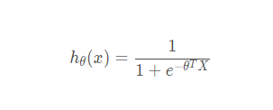
Hypothesis function and cost function of logistic regression

Sigmoid function

#  Hypothesis function of logistic regression
def sigmoid(z):
    return 1 / (1 + np.exp(-z))
# Test it to ensure the correctness of the Sigmoid function
# x1 = np.arange(-10, 10, 1)
# plt.plot(x1, sigmoid(x1), c='r')
# plt.show()

Cost Function

The cost function of logistic regression is as follows, which is different from that of linear regression because this function is convex.

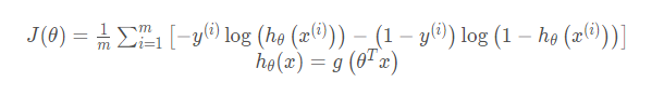
# Cost function
def cost(theta, X, y):
    first = (-y) * np.log(sigmoid(X @ theta))
    second = (1 - y) * np.log(1 - sigmoid(X @ theta))
    return np.mean(first - second)
# Test cost, and be sure to find the corresponding relationship when vectorizing
# a = cost(theta, X, y)   # 0.6931471805599453
# print(a)

Gradient function

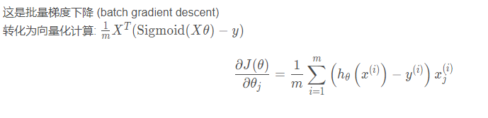
# print((X.T @ (sigmoid(X @ theta) - y)).shape) # (3,)
# Convert to vector operation, pay attention to the transpose problem @ equivalent dot()
def gradient(theta, X, y):
    return (X.T @ (sigmoid(X @ theta) - y)) / len(X)
# print(gradient(theta, X, y)) # [ -0.1        -12.00921659 -11.26284221]

Optimization

We're not actually doing gradient descent in this function, we're just calculating the gradient. In the exercise, an Octave function called "fminunc" is used to optimize the function to calculate cost and gradient parameters. Since we use Python, we can do the same thing with SciPy's "optimize" namespace.
Here we use advanced optimization algorithms, which usually run much faster than gradient descent. Convenient and fast.
Just pass in the cost function, the variable theta, and the gradient. When the cost function defines a variable, the variable tehta should be placed first. If the cost function only returns cost, set fprime=gradient.

# res is used to return the appropriate n different theta in the parametric equation_ I value
res = opt.minimize(fun=cost, x0=theta, jac=gradient, args=(X, y), method='TNC')
# res2 = opt.fmin_tnc(func=cost, x0=theta, fprime=gradient, args=(X, y))
# print(res)
# print(res2)

     fun: 0.203497701589475
     jac: array([9.14875519e-09, 9.99037356e-08, 4.79345707e-07])
 message: 'Local minimum reached (|pg| ~= 0)'
    nfev: 36
     nit: 17
  status: 0
 success: True
       x: array([-25.16131853,   0.20623159,   0.20147149])

res.x is the desired theta

Operation model

function

Hypothetical function of logistic regression model:

def predict(theta, X):
    probablility = sigmoid(X @ theta)
    return [1 if x >= 0.5 else 0 for x in probablility] # Returns a list
predictions = predict(res.x, X)
# print(predictions)

# Comparative accuracy
correct = []
for i in range(len(predictions)):
    if predictions[i] == y[i]:
        correct.append(1)
    else:
        correct.append(0)
    pass
accuracy = sum(correct)/len(X)
print("Accuracy detection is===>", accuracy) # 0.89

Method detection in sklearn

'''
4.sklearn To test
'''
print("sklearn To test===>", classification_report(predictions, y))

Drawing

'''
4.Drawing
'''
# The following is determined according to the mathematical relationship
x1 = np.arange(130, step=0.1) # Abscissa
x2 = -(res.x[0] + x1 * res.x[1]) / res.x[2] # Ordinate
fig2, ax = plt.subplots(figsize=(8, 6))
ax.scatter(positive['exam1'], positive['exam2'], c='orange', label='Admitted')
ax.scatter(negetive['exam1'], negetive['exam2'], c='b', marker='*', label='Not Admitted')
ax.plot(x1, x2)
ax.set_xlim(0, 130)
ax.set_ylim(0, 130)
ax.set_xlabel('x1')
ax.set_ylabel('x2')
ax.set_title('Decision boundary')
plt.show()

Assignment topic 2 regulated logistic regression

We will improve the logistic regression algorithm by adding regular terms. In short, regularization is a term in the cost function, which makes the algorithm prefer a "simpler" model (in this case, the model will have smaller coefficients). This theory helps to reduce over fitting and improve the generalization ability of the model. Well, let's start.

Imagine that you are the production supervisor of the factory, and you have the test results of some chips in two tests. For these two tests, you want to decide whether the chip will be accepted or discarded. To help you make difficult decisions, you have a test data set of past chips from which you can build a logistic regression model.

Feature mapping

A better way to fit data is to create more features from each data point. We will map these features to all polynomial terms of x1 and x2.

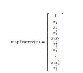
def featureMapping(x1, x2, power):
    data = {}
    # data here is a dictionary
    for i in np.arange(power + 1):
        for p in np.arange(i + 1):
            data["f{}{}".format(i - p, p)] = np.power(x1, i-p) * np.power(x2, p)
            pass
    # Assuming power=3, columns 00, 10, 01, 20, 11, 02, 30, 21, 12 and 03 will be formed in the dictionary
    return pd.DataFrame(data)

	x1 = np.array(data2['Test 1'])
	x2 = np.array(data2['Test 2'])
	_data2 = featureMapping(x1, x2, 7)
	# print(_data2)

After mapping, we transform the vector with two features into a 36 dimensional vector.

The logistic regression classifier trained on this high-dimensional feature vector will have a more complex decision boundary. When we draw it in a two-dimensional graph, it will be nonlinear.

Although feature mapping allows us to build a more expressive classifier, it is also easier to over fit. In the next exercise, we will implement regularized logistic regression to fit the data, and we can see how regularization can help solve the problem of over fitting.
Processing data

# First obtain the feature, label and parameter theta to ensure that the dimension is good
X = np.array(_data2)
y = np.array(data2['Accepted'])
theta = np.zeros(X.shape[1])
print(X.shape, y.shape, theta.shape)

Regularized Cost Funciton

Note: the first item will not be punished θ 0

All codes

# Kyrie Irving
# !/9462...
import numpy as np
import pandas as pd
import matplotlib.pyplot as plt
import scipy.optimize as opt
from sklearn.metrics import classification_report
from sklearn import linear_model    # Call the linear regression package of sklearn

'''
Prepare data
'''
def preparData():
    data2 = pd.read_csv('ex2data2.txt', names=['Test 1', 'Test 2', 'Accepted'])
    # print(data2.head())
    return data2

'''
Visualize existing data
'''
def plotData(data2):
    # Classified data, separating admission and non admission
    positive = data2[data2.Accepted.isin([1])]  # 1
    negetive = data2[data2.Accepted.isin([0])]  # 0

    fig, ax = plt.subplots(figsize=(8, 6))
    ax.scatter(positive['Test 1'], positive['Test 2'], c='orange', label='Admitted')
    ax.scatter(negetive['Test 1'], negetive['Test 2'], c='b', marker='*', label='Not Admitted')
    # The setting legend is displayed at the top of the diagram
    box = ax.get_position()
    # If the legend is drawn outside the coordinates, if it is placed on the right, generally give a value of about width*0.8, and on the top, give a value of about height*0.8
    ax.set_position([box.x0, box.y0, box.width, box.height * 0.8])
    ax.legend(loc='center left', bbox_to_anchor=(0.2, 1.12), ncol=2)
    '''
    (Look right horizontally and down vertically),If you want to customize the legend position or draw the legend outside the coordinates, use it,
    such as bbox_to_anchor=(1.4,0.8)，This generally matches ax.get_position()，set_position([box.x0, box.y0, box.width*0.8 , box.height])use
    Unused parameters can be removed directly,Some parameters are not written in, and they are added if available , bbox_to_anchor=(1.11,0)
    '''
    '''
    # Set the abscissa and ordinate names
    ax.set_xlabel('Test 1')
    ax.set_ylabel('Test 2')
    plt.show()

'''
Feature scaling
'''
def featureMapping(x1, x2, power):
    data = {}
    # data here is a dictionary
    for i in np.arange(power + 1):
        for p in np.arange(i + 1):
            data["f{}{}".format(i - p, p)] = np.power(x1, i-p) * np.power(x2, p)
            pass
    # Assuming power=3, columns 00, 10, 01, 20, 11, 02, 30, 21, 12 and 03 will be formed in the dictionary
    return pd.DataFrame(data)

'''
Processing data
'''
def dealData(_data2, data2):
    # First obtain the feature, label and parameter theta to ensure that the dimension is good
    X = np.array(_data2)
    y = np.array(data2['Accepted'])
    theta = np.zeros(X.shape[1])
    # print(X.shape, y.shape, theta.shape)
    return X, y, theta

'''
The following are the conditional equations
'''
# 1)Sigmoid Fuc
def sigmoid(z):
    return 1 / (1 + np.exp(-z))

# 2)Cost Fuc
def cost(theta, X, y):
    first = (-y) * np.log(sigmoid(X @ theta))
    second = (1 - y)*np.log(1 - sigmoid(X @ theta))
    return np.mean(first - second)

def gradient(theta, X, y):
    # the gradient of the cost is a vector of the same length as θ where the jth element (for j = 0, 1, . . . , n)
    return (X.T @ (sigmoid(X @ theta) - y)) / len(X)

def costReg(theta, X, y, Lambda):
    # Do not punish the first item (remove item 0)
    _theta = theta[1:]
    reg = (Lambda/2*len(X))*(_theta @ _theta)   # _theta@_theta == inner product
    return cost(theta, X, y) + reg

def gradientReg(theta, X, y, Lambda):
    reg = (Lambda/len(X)) * theta
    reg[0] = 0
    return gradient(theta, X, y) + reg

def predict(theta, X):
    probability = sigmoid(X @ theta)
    return [1 if x >= 0.5 else 0 for x in probability]  # return a list

if __name__ == '__main__':
    data2 = preparData()
    # plotData(data2) # Display data

    x1 = np.array(data2['Test 1'])
    x2 = np.array(data2['Test 2'])
    _data2 = featureMapping(x1, x2, 7) # The scaled data is transformed into a 36 dimensional (column) vector
    # print(_data2)

    X, y, theta = dealData(_data2, data2) # First obtain the feature, label and parameter theta to ensure good dimension
    # print(X)
    # print(y)
    # print(theta)
    a = costReg(theta, X, y, 1)  # 0.6931471805599454 at this time θ All 0
    b = gradientReg(theta, X, y, 1)
    # print(b)

    res = opt.minimize(fun=costReg, x0=theta, jac=gradientReg, args=(X, y, 1), method='TNC')
    print(res)

    model = linear_model.LogisticRegression(penalty='l2', C=1.0)
    model.fit(X, y.ravel())
    print(model.score(X, y))

    '''
    -Evaluating logistic regression
    '''
    final_theta = res.x
    predictions = predict(final_theta, X)
    # 1
    correct = [1 if a == b else 0 for (a, b) in zip(predictions, y)]
    accuracy = sum(correct) / len(correct)
    print("logistic Evaluation accuracy of hypothetical function of regression===>", accuracy)
    # 2
    print("sklearn To evaluate accuracy===>", classification_report(y, predictions))

    '''
    -Decision boundary
    '''
    x = np.linspace(-1, 1.5, 150)
    xx, yy = np.meshgrid(x, x)
    # Generate a grid diagram composed of X. the abscissa X and ordinate y return the abscissa xx and ordinate YY 150150 of the network coordinate points intersected by all lines after passing through the meshgrid(x,y)
    # xx. Convert travel() to one-dimensional data
    z = np.array(featureMapping(xx.ravel(), yy.ravel(), 7))

    z = z @ final_theta
    z = z.reshape(xx.shape)

    plotData(data2)
    plt.contour(xx, yy, z, 0)
    plt.ylim(-0.8, 1.2)
    plt.show()