preface
Follow the previous section Point cloud 1
Data address of this section: link: https://pan.baidu.com/s/1O4s8tFOvExhuKMl2OCv4Kg
Extraction code: 82u1
1. Point cloud clipping
Code first
import open3d as o3d

pcd=o3d.io.read_point_cloud("./test_data/Crop/fragment.ply")
val=o3d.visualization.read_selection_polygon_volume("./test_data/Crop/cropped.json")
chair=val.crop_point_cloud(pcd)
o3d.visualization.draw_geometries([chair],
                                  zoom=0.7,
                                  front=[0.5439, -0.2333, -0.8060],
                                  lookat=[2.4615, 2.1331, 1.338],
                                  up=[-0.1781, -0.9708, 0.1608])
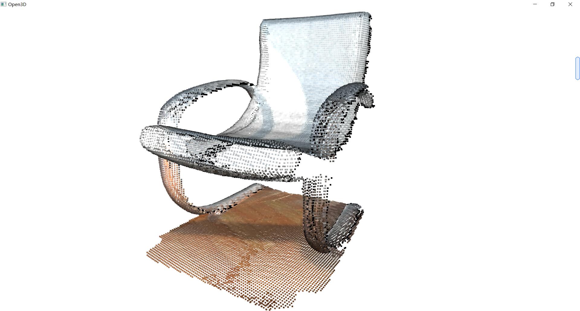
o3d. visualization. read_ selection_ polygon_ The volume function initializes an O3D. Net file based on the read file visualization. Selectionpolygonvolume(), this object is used to crop the point cloud. The crop of the object_ point_ The cloud method is used to clip the point cloud. The input is the point cloud to be cropped.
The clipping results are as follows:
2. Point cloud bounding box
import open3d as o3d
pcd=o3d.io.read_point_cloud("../test_data/Crop/fragment.ply")
vol=o3d.visualization.read_selection_polygon_volume("../test_data/Crop/cropped.json")
chair=vol.crop_point_cloud(pcd)
aadd=chair.get_axis_aligned_bounding_box()
aadd.color=(1,0,0)
obb=chair.get_oriented_bounding_box()
obb.color=(0,1,0)
o3d.visualization.draw_geometries([chair,aadd,obb],
                                  zoom=0.7,
                                  front=[0.5439, -0.2333, -0.8060],
                                  lookat=[2.4615, 2.1331, 1.338],
                                  up=[-0.1781, -0.9708, 0.1608]
                                  )
Here, we first cut out the chair in the point cloud, and then calculate the two kinds of bounding boxes of the chair. Get of point cloud object_ axis_ aligned_ bounding_ The box method calculates the minimum axis alignment bounding box of the point cloud. get_ oriented_ bounding_ The box method returns the oriented bounding box of the geometry. Both methods return O3D geometry. Axisalignedboundingbox object, which is used to record the object of the bounding box.
3. Convex hull
The convex hull of a point cloud is the smallest convex set containing all points. Open3D contains the method of calculating the convex hull of a point cloud. The implementation is based on Qhull.
import open3d as o3d

pcl = o3d.io.read_triangle_mesh("./test_data/bun_zipper.ply")
o3d.visualization.draw_geometries([pcl],window_name="mesh",width=810,height=520)
pcl=pcl.sample_points_poisson_disk(number_of_points=2000)
o3d.visualization.draw_geometries([pcl],window_name="pointcloud",width=810,height=520)
#Creates a convex hull and returns the convex hull vertices
hull, _ = pcl.compute_convex_hull()
#Connect vertices of convex hull
hull_ls = o3d.geometry.LineSet.create_from_triangle_mesh(hull)
hull_ls.paint_uniform_color((1, 0, 0))
o3d.visualization.draw_geometries([pcl, hull_ls])
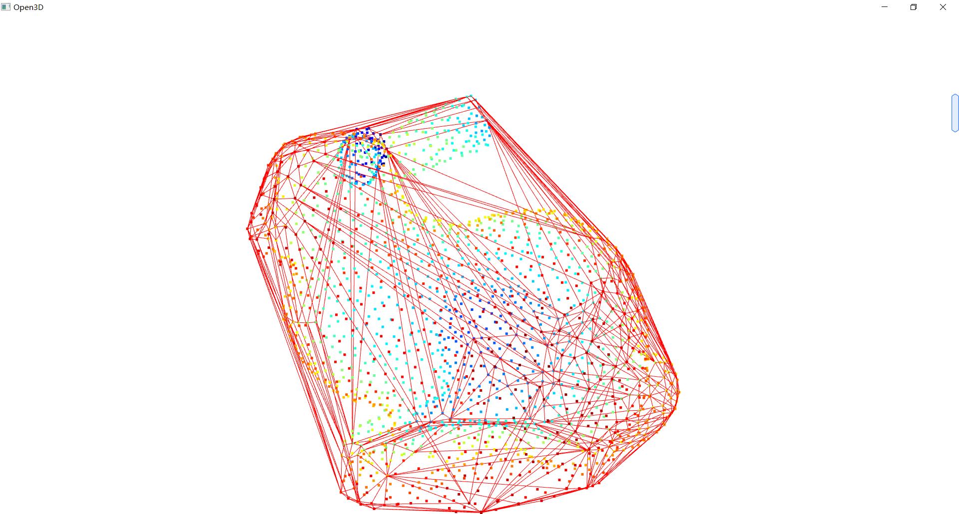
Code analysis: O3D io. read_ triangle_ Mesh is used to read triangular mesh data. Then let's visualize the triangular mesh data. Sample using triangular mesh objects_ points_ poisson_ The disk method samples the triangular mesh into a point cloud, and the input parameter is the number of points of the point cloud after sampling. Then use the compute of the point cloud object_ convex_ Hull method is used to calculate the convex hull of point cloud. Then use O3D geometry. LineSet. create_ from_ triangle_ The mesh function creates a line set from a convex hull. Finally, render the line set in red.
The visualization results are as follows:
4.DBSCAN clustering
Given a point cloud from, for example, a depth sensor, we want to group the point cloud clusters together. To this end, we can use clustering algorithm. Open3D implements DBSCAN, a density based clustering algorithm.
The code is as follows:
import open3d as o3d
import numpy as np
import matplotlib.pyplot as plt

pcd=o3d.io.read_point_cloud("./test_data/fragment.ply")
o3d.visualization.draw_geometries([pcd],window_name="before cluster",width=810,height=520,
                                  zoom=0.455,
                                  front=[-0.4999, -0.1659, -0.8499],
                                  lookat=[2.1813, 2.0619, 2.0999],
                                  up=[0.1204, -0.9852, 0.1215])
with o3d.utility.VerbosityContextManager(o3d.utility.VerbosityLevel.Debug) as cm:
    label=np.array(pcd.cluster_dbscan(eps=0.02,min_points=10,print_progress=True))

#Cluster number
max_label=label.max()
print(f"point cloud has {max_label + 1} clusters")
colors=plt.get_cmap("tab20")(label/(max_label if max_label>0 else 1))
colors[label<0]=0
pcd.colors=o3d.utility.Vector3dVector(colors[:,:3])
o3d.visualization.draw_geometries([pcd],window_name="after cluster",width=810,height=520,
                                  zoom=0.455,
                                  front=[-0.4999, -0.1659, -0.8499],
                                  lookat=[2.1813, 2.0619, 2.0999],
                                  up=[0.1204, -0.9852, 0.1215]
                                  )
Code parsing:
Of which O3D utility. The verbositycontextmanager object is the context manager of open3d. Cluster of point cloud objects_ DBSCAN method implements DBSCAN clustering.
cluster_ Parameters of DBSCAN method:
eps: used to find density parameters belonging to a cluster
min_points: the minimum number of points forming a cluster.
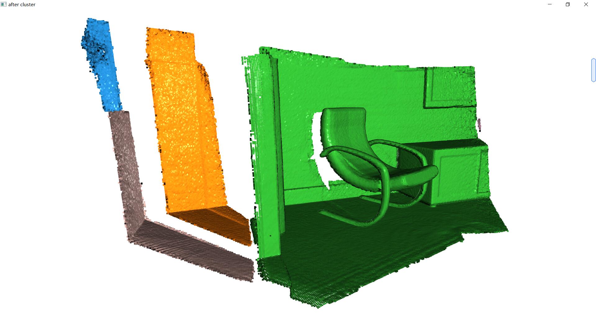
Then get the number of clusters and use PLT get_ CMAP renders different colors for each cluster.
The visualization results are as follows:
5. Plane segmentation
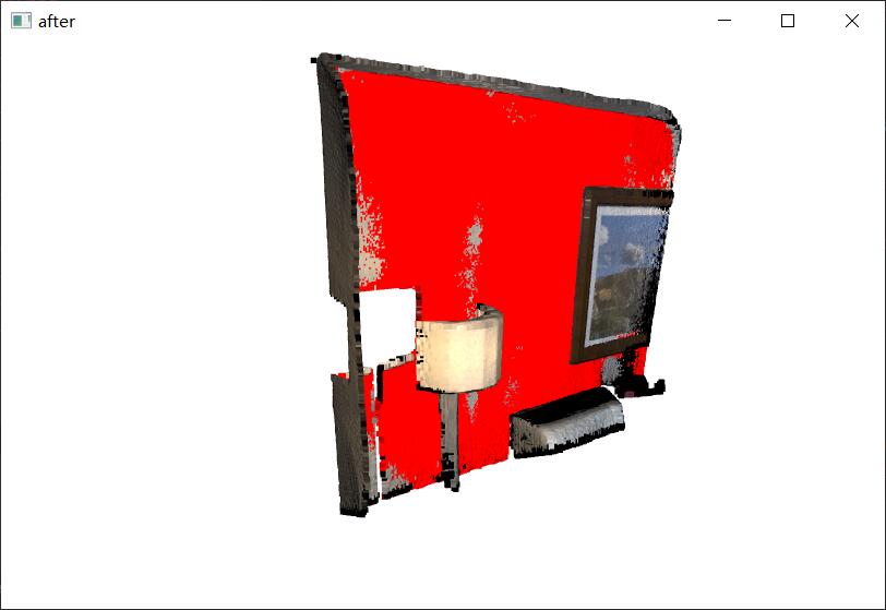
We use RANSAC to segment the geometric primitives in the point cloud to find the maximum support plane in the point cloud.
The code is as follows:
import open3d as o3d

pcd=o3d.io.read_point_cloud("./test_data/fragment.pcd")
o3d.visualization.draw_geometries([pcd],window_name="Initial point cloud",
                                  width=810,height=520,
                                  zoom=0.8,
                                  front=[-0.4999, -0.1659, -0.8499],
                                  lookat=[2.1813, 2.0619, 2.0999],
                                  up=[0.1204, -0.9852, 0.1215])
#Plane estimation returns the estimated plane parameters and the index of the point cloud plane
plane_model,inliers=pcd.segment_plane(distance_threshold=0.01,
                                      ransac_n=3,
                                      num_iterations=1000)
#Take out parameters
[a,b,c,d]=plane_model
print(f"Plane equation: {a:.2f}x + {b:.2f}y + {c:.2f}z + {d:.2f} = 0")
#Cable lead out plane
inlier_cloud=pcd.select_by_index(inliers)
inlier_cloud.paint_uniform_color([1.0,0,0])
o3d.visualization.draw_geometries([inlier_cloud],window_name="inlier_cloud",
                                  width=810,height=520,
                                  zoom=0.8,
                                  front=[-0.4999, -0.1659, -0.8499],
                                  lookat=[2.1813, 2.0619, 2.0999],
                                  up=[0.1204, -0.9852, 0.1215])
#Points outside the plane
outlier_cloud=pcd.select_by_index(inliers,invert=True)
o3d.visualization.draw_geometries([outlier_cloud],window_name="outlier_cloud",
                                  width=810,height=520,
                                  zoom=0.8,
                                  front=[-0.4999, -0.1659, -0.8499],
                                  lookat=[2.1813, 2.0619, 2.0999],
                                  up=[0.1204, -0.9852, 0.1215])
o3d.visualization.draw_geometries([inlier_cloud,outlier_cloud],window_name="after",
                                  width=810,height=520,
                                  zoom=0.8,
                                  front=[-0.4999, -0.1659, -0.8499],
                                  lookat=[2.1813, 2.0619, 2.0999],
                                  up=[0.1204, -0.9852, 0.1215]
                                  )
Code parsing:
Segment of point cloud object_ The plane method uses the RANSAC algorithm to segment the plane in the point cloud.
The parameters are as follows:
distance_threshold: the distance between the point cloud and the plane is less than this distance. This point is regarded as the inner point of the plane
ransac_n: The number of initial points to be inlined should be considered in each iteration
num_iterations: iterations
Seed: seed value used in the random generator
This function returns a tuple. The first element is the parameter of the plane, and the second element is the list composed of the point index of the maximum support surface of the point cloud.
Then we use the select of the point cloud object_ by_ Index method takes out the point cloud of the maximum support plane. The first parameter of this method is the point cloud index. When the second parameter invert is True, it is the reverse index, which leads to the points other than the input point cloud index.
We render the maximum support plane red.
The visualization results are as follows:
Hidden point removal
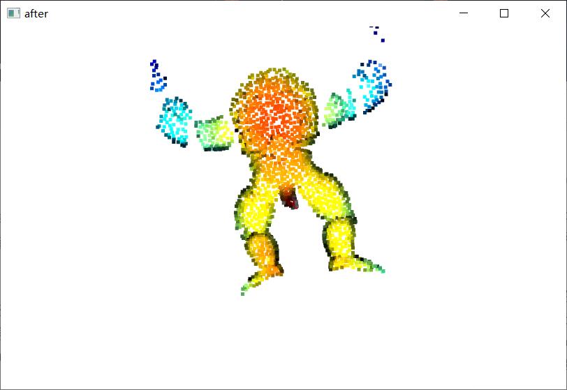
Simply put, it is to observe the point cloud from a viewpoint and remove the invisible points
The code is as follows:
import open3d as o3d
import numpy as np
#Load point cloud in the way of triangular mesh
pcd=o3d.io.read_triangle_mesh("./test_data/Armadillo.ply")
#Estimating the normals of triangular meshes
pcd.compute_vertex_normals()
#Sample triangular meshes into point clouds
pcd=pcd.sample_points_poisson_disk(5000)
#Calculation norm, geometric maximum boundary and minimum boundary
diameter=np.linalg.norm(np.asarray(pcd.get_max_bound())-np.asarray(pcd.get_min_bound()))
o3d.visualization.draw_geometries([pcd],window_name="Initial point cloud",
                                  width=810,height=520,
                                  zoom=0.8,
                                  front=[-0.4999, -0.1659, -0.8499],
                                  lookat=[2.1813, 2.0619, 2.0999],
                                  up=[0.1204, -0.9852, 0.1215])
print("Define parameters used for hidden_point_removal")
#Parameters for hidden point deletion
camera = [0, 0, diameter]
radius=diameter*100
#Gets all points visible from the viewpoint
print("Get all points that are visible from given view point")
_,ptmap=pcd.hidden_point_removal(camera,radius)

pcd=pcd.select_by_index(ptmap)
o3d.visualization.draw_geometries([pcd],window_name="after",
                                  width=810,height=520,
                                  zoom=0.8,
                                  front=[-0.4999, -0.1659, -0.8499],
                                  lookat=[2.1813, 2.0619, 2.0999],
                                  up=[0.1204, -0.9852, 0.1215])
Code parsing:
Compute of triangular mesh object_ vertex_ The normals method is used to estimate the vertex normals of triangular meshes.
Hidden of point cloud objects_ point_ The removal method realizes the removal of hidden points
The parameters are as follows:
camera_location: is the viewpoint
Radius: projection radius
This function also returns a tuple. The second element of the tuple is the index of all points visible from a given viewpoint, and then we index the visible point cloud.
The visualization results are as follows:
