Original address

original text

Thesis reading methods

Three times thesis method

First acquaintance

CNN method is brilliant in the field of computer vision, and has replaced the traditional method in many fields. However, the architecture of convolutional neural network lacks spatial invariance. Even if convolution and Max pooling operations introduce translation invariance and spatial invariance to a certain extent, CNN will become unrecognizable if the input changes greatly in space.

Therefore, this paper proposes a spatial transformation module and constructs a spatial transformation network, which can increase the spatial invariance of CNN to a certain extent. And this is a plug and play module, which can be easily inserted into various architectures.

Acquaintances

The main technology and some experiments are introduced

Spatial transformation based on matrix operation

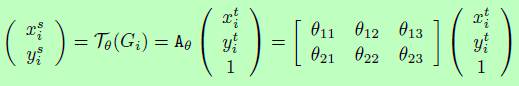
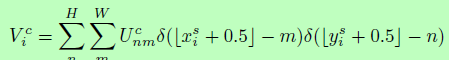
Small partners familiar with traditional image processing must know that most spatial transformations can be converted into matrix based sampling operations. It is assumed that the pixels of the input image (source) are generated by( x i s , y i s x_i^s, y_i^s xis, yis) indicates that the output image (target) pixel is composed of( x i t , y i t x_i^t, y_i^t xit, yit) means that as long as a set of transformation parameters is determined θ You can determine a spatial transformation. Take 2D radiation transformation matrix as an example:

matrix A θ A_θ A θ There can be translation, rotation, scaling, staggered cutting and other operations. As long as six parameters are determined, the values of each pixel of the output image can be obtained according to the matrix transformation (regarded as the operation of sampling from the original image).

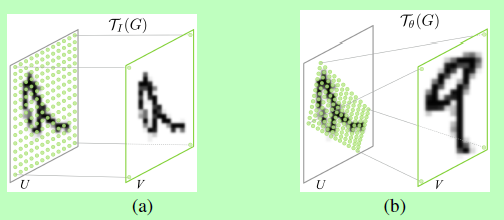
The identity map is pasted here( θ 11 , θ 22 θ_{11}, θ_{22} θ 11​, θ 22 ￠ is 1 (others are 0) and an affine change effect diagram:

For more information about 2D affine transformation matrix, please refer to this article: Understanding of affine transformation and its transformation matrix

Since the spatial transformation can be determined as matrix operation, it is advisable to let the network learn to generate matrix parameters, so as to learn spatial transformation.

Overall architecture

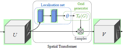
The overall structure of the STN module is shown in the figure above. It is composed of localization net, Grid generator and Sampler. The input feature map U (or RGB image directly) is obtained through the spatial transformation module to obtain the output feature map V.

Localization net sends the input characteristic map to a subnet to obtain the spatial variation parameters θ； Grid generator according to θ Determine a spatial change and create a sampling grid to determine which points in the input graph will be used for transformation; The Sampler samples the input characteristic graph according to the sampling grid to obtain the final output.

Localisation net

The positioning subnet receives the input feature map, sends it to the hidden layer to extract features (which can be convolution layer or full connection layer), and outputs the corresponding parameters according to the preset transformation (for example, the affine transformation mentioned earlier is 6 parameters).

Grid generator

In fact, the transformation matrix is constructed according to the parameters to determine the sampling space.

There are some details to note. The coordinates of the input and output diagrams are normalized to [- 1,1]

Image Sampling

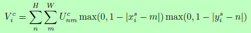
If you want to learn network parameters by gradient descent method, you must pay attention to the derivability of operation. The sampling operation itself is not differentiable, because the input pixels are discrete, and the spatial conversion will cause the sampling points not to be the pixel values on the original image. Therefore, the author introduces the interpolation operation to make the process derivable:

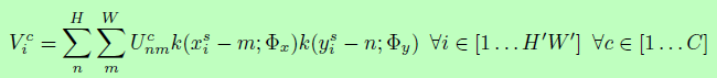
Where U is the input characteristic diagram, V is the output characteristic diagram, and k is the interpolation operation.

Thus, the nearest neighbor interpolation and bilinear interpolation are as follows:

The interpolation process is derivable, and the partial derivation process is as follows:

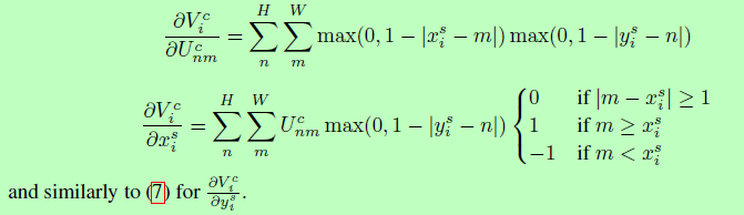
Therefore, the whole module can update the parameters through the back propagation algorithm, so as to be embedded into the network for end-to-end training.

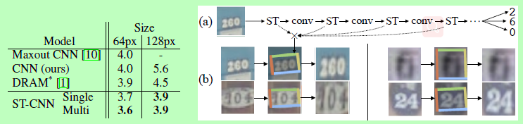
Partial experiment

① Some disturbances are made to MNIST data, which makes it difficult to distinguish normal CNN. After introducing STN module, it can be recognized normally after transformation.

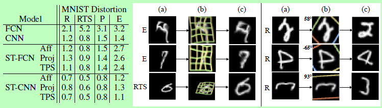
② In the house number recognition, multiple STN structure is introduced to improve the recognition performance.

review

STN has been working for 15 years, but its thought has also affected a large number of later work. The main highlight is that the spatial transformation is transformed into a parameter prediction, and then sampled by interpolation, so that it can be embedded into the network for end-to-end training.

But its performance is not as good as the legend, nor can it replace the role of random amplification. Because there is no direct constraint on the spatial transformation, you can't expect it to achieve the transformation form you want. For example, in the MNIST experiment, the reason why it can learn to restore the inverted 4 transform is that most of the training data of the whole category are positive. If your whole category is the inverted 4, it cannot learn, and its parameter update depends on your overall training goal.

I have used this module in the image classification competition and expect it to play a role similar to Attention to enlarge the key information in the image, but the experimental effect is not good.

code

Pytoch has encapsulated the two main operations of STN network generation sampling network + sampling into torch.nn.funcitonal, so the reproduction is relatively simple.

The following code mainly shows the STN module, in which localisation net can be modified according to specific tasks and data. The default input image dimension here is 512x512x3:

# Down sampling module based on convolution
def ConvBnRelu(in_channel, out_channel):
    convbnrelu = nn.Sequential(
        nn.Conv2d(in_channel, out_channel, kernel_size=3, stride=2, padding=1),
        nn.BatchNorm2d(out_channel),
        nn.ReLU(inplace=True)
    )
    return convbnrelu


class SpatialTransformer(nn.Module):
    """ Spatial Transformer Network """
    def __init__(self):
        super(SpatialTransformer, self).__init__()
        self.localization = nn.Sequential(
            # Conv-Bn-Relu (downsampling)
            ConvBnRelu(3, 64),
            ConvBnRelu(64, 128),
            ConvBnRelu(128, 256),
            ConvBnRelu(256, 512),
            nn.Conv2d(512, 256, kernel_size=1, bias=False),
            nn.Conv2d(256, 1, kernel_size=1, bias=False)
        )
		# Location subnet
        self.fc_loc = nn.Sequential(
            nn.Linear(32*32, 128),
            nn.BatchNorm1d(128),
            nn.ReLU(inplace=True),
            nn.Linear(128, 2*3)
        )
        # initialization
        for m in self.modules():
            if isinstance(m, nn.Conv2d):
                nn.init.kaiming_normal_(m.weight, mode='fan_out', nonlinearity='relu')
            elif isinstance(m, (nn.BatchNorm2d, nn.GroupNorm)):
                nn.init.constant_(m.weight, 1)
                nn.init.constant_(m.bias, 0)
        # Identity transformation initialization identity mapping
        self.fc_loc[3].weight.data.fill_(0)
        self.fc_loc[3].bias.data = torch.FloatTensor([1, 0, 0, 0, 1, 0])

    def forward(self, img):

        n = img.shape[0]

        feature = self.localization(img).flatten(start_dim=1)
        theta = self.fc_loc(feature).reshape(n, 2, 3)

        # spatial transform
        grid = F.affine_grid(theta, size=img.size(), align_corners=False)
        trans_img = F.grid_sample(img, grid, align_corners=False)

        return trans_img