Supervised learning is a traditional method of training machine learning model. During training, every observed data needs to be labeled. What if we had a way to train machine learning models without collecting labels? What if we extract tags from the same data collected? This type of learning algorithm is called self supervised learning. This method works well in natural language processing. An example is BERT ¹, Google has been using BERT in its search engine since 2019 ¹. Unfortunately, this is not the case for computer vision.
kaiming great God of Facebook AI and others proposed a masked self encoder (MAE) ², It is based on (ViT) ³ framework. Their method performs better on ImageNet than vit trained from scratch. In this article, we'll delve into their approach and see how to implement it in code.
Masked self encoder (MAE)
The patches of the input image are randomly masked, and then the missing pixels are reconstructed. MAE is based on two core designs. Firstly, an asymmetric encoder decoder architecture is developed, in which the encoder only operates on the subset of visible patches (unmasked tokens). At the same time, there is a lightweight decoder that can reconstruct the original image from potential representations and masked tokens. Secondly, it is found that masking the input image with a high proportion, such as 75%, will produce a meaningful self-monitoring task. Combining these two designs can efficiently train large models: speed up model training (3 times or more) and improve accuracy.

This stage is called pre training because the MAE model will later be used for downstream tasks, such as image classification. The performance of the model on pretext is not important in self-monitoring. The focus of these tasks is to let the model learn an intermediate representation that is expected to contain good semantics. After the pre training phase, the decoder will be replaced by multi-layer perceptron (MLP) head or linear layer as a classifier to output the prediction of downstream tasks.

Model architecture
encoder
The encoder is ViT. It accepts images with tensor shape (batch_size, RGB_channels, height, width). Embedding is obtained for each Patch by performing linear projection, which is completed by 2D convolution layer. Then the tensor is flattened (flattened) in the last dimension and becomes (batch_size, encoder_embedded_dim, num_visible_patches) and transposed to the tensor of shape (batch_size, num_visible_patches, encoder_embedded_dim).
class PatchEmbed(nn.Module):
    """ Image to Patch Embedding """
    def __init__(self, img_size=(224, 224), patch_size=(16, 16), in_chans=3, embed_dim=768):
        super().__init__()
        self.img_size = img_size
        self.patch_size = patch_size
        self.num_patches = (img_size[1] // patch_size[1]) * (img_size[0] // patch_size[0])
        self.patch_shape = (img_size[0] // patch_size[0], img_size[1] // patch_size[1])
        self.proj = nn.Conv2d(in_chans, embed_dim, kernel_size=patch_size, stride=patch_size)

    def forward(self, x, **kwargs):
        B, C, H, W = x.shape
        assert H == self.img_size[0] and W == self.img_size[1], f"Input image size ({H}*{W}) doesn't match model ({self.img_size[0]}*{self.img_size[1]})."
        x = self.proj(x).flatten(2).transpose(1, 2)
        return x
As mentioned in the original Transformer paper, location coding adds information about each Patch location. The author uses the "sine cosine" version instead of learnable location embedding. The following implementation is a one-dimensional version.
def get_sinusoid_encoding_table(n_position, d_hid):

    def get_position_angle_vec(position):
        return [position / np.power(10000, 2 * (hid_j // 2) / d_hid) for hid_j in range(d_hid)]

    sinusoid_table = np.array([get_position_angle_vec(pos_i) for pos_i in range(n_position)])
    sinusoid_table[:, 0::2] = np.sin(sinusoid_table[:, 0::2]) # dim 2i
    sinusoid_table[:, 1::2] = np.cos(sinusoid_table[:, 1::2]) # dim 2i+1
    return torch.FloatTensor(sinusoid_table).unsqueeze(0)
Similar to Transformer, each block is composed of norm layer, multi head attention module and feedforward layer. The intermediate output shapes are (batch_size, num_visible_patches, encoder_embedded_dim). The code of multi head attention module is as follows:
class Attention(nn.Module):
    def __init__(self, dim, num_heads=8, qkv_bias=False, qk_scale=None, attn_drop=0., proj_drop=0., attn_head_dim=None):
        super().__init__()
        self.num_heads = num_heads
        head_dim = attn_head_dim if attn_head_dim is not None else dim // num_heads
        all_head_dim = head_dim * self.num_heads
        self.scale = qk_scale or head_dim ** -0.5
        self.qkv = nn.Linear(dim, all_head_dim * 3, bias=False)
        self.q_bias = nn.Parameter(torch.zeros(all_head_dim)) if qkv_bias else None
        self.v_bias = nn.Parameter(torch.zeros(all_head_dim)) if qkv_bias else None
        self.attn_drop = nn.Dropout(attn_drop)
        self.proj = nn.Linear(all_head_dim, dim)
        self.proj_drop = nn.Dropout(proj_drop)

    def forward(self, x):
        B, N, C = x.shape
        qkv_bias = torch.cat((self.q_bias, torch.zeros_like(self.v_bias, requires_grad=False), self.v_bias)) if self.q_bias is not None else None
        qkv = F.linear(input=x, weight=self.qkv.weight, bias=qkv_bias)
        qkv = qkv.reshape(B, N, 3, self.num_heads, -1).permute(2, 0, 3, 1, 4)
        q, k, v = qkv[0], qkv[1], qkv[2]   # make torchscript happy (cannot use tensor as tuple)
        q = q * self.scale
        attn = (q @ k.transpose(-2, -1)).softmax(dim=-1)
        attn = self.attn_drop(attn)
        x = (attn @ v).transpose(1, 2).reshape(B, N, -1)
        x = self.proj_drop(self.proj(x))
        return x
The code of Transformer module is as follows:
class Block(nn.Module):
    def __init__(self, dim, num_heads, mlp_ratio=4., qkv_bias=False, qk_scale=None, drop=0., attn_drop=0.,act_layer=nn.GELU, norm_layer=nn.LayerNorm, attn_head_dim=None):
        super().__init__()
        self.norm1 = norm_layer(dim)
        self.attn = Attention(
            dim, num_heads=num_heads, qkv_bias=qkv_bias, qk_scale=qk_scale,
            attn_drop=attn_drop, proj_drop=drop, attn_head_dim=attn_head_dim)
        self.norm2 = norm_layer(dim)
        self.mlp = nn.Sequential(
            nn.Linear(dim, int(dim * mlp_ratio)), act_layer(), nn.Linear(int(dim * mlp_ratio), dim), nn.Dropout(attn_drop)
        )

    def forward(self, x):
        x = x + self.attn(self.norm1(x))
        x = x + self.mlp(self.norm2(x))
        return x
This section is only used for fine tuning of downstream tasks. The model of this paper follows the ViT architecture, which has a class token (patch) for classification. Therefore, they added a virtual token, but the paper also said that their method can work well without it because it performs an average pooling operation on other tokens. The average pooled version of the implementation is also included here. After that, a linear layer is added as a classifier. The final tensor shape is (batch_size, num_classes).
To sum up, the encoder is implemented as follows:
class Encoder(nn.Module)
    def __init__(self, img_size=224, patch_size=16, in_chans=3, embed_dim=768, norm_layer=nn.LayerNorm, num_classes=0, **block_kwargs):
        super().__init__()
        self.num_classes = num_classes
        self.num_features = self.embed_dim = embed_dim  # num_features for consistency with other models

        # Patch embedding
        self.patch_embed = PatchEmbed(img_size=img_size, patch_size=patch_size, in_chans=in_chans, embed_dim=embed_dim)
        num_patches = self.patch_embed.num_patches

        # Positional encoding
        self.pos_embed = get_sinusoid_encoding_table(num_patches, embed_dim)

        # Transformer blocks
        self.blocks = nn.ModuleList([Block(**block_kwargs) for i in range(depth)])  # various arguments are not shown here for brevity purposes
        self.norm =  norm_layer(embed_dim)

        # Classifier (for fine-tuning only)
        self.fc_norm = norm_layer(embed_dim)
        self.head = nn.Linear(embed_dim, num_classes)

    def forward(self, x, mask):
        x = self.patch_embed(x)
        x = x + self.pos_embed.type_as(x).to(x.device).clone().detach()
        B, _, C = x.shape
        if mask is not None:  # for pretraining only
            x = x[~mask].reshape(B, -1, C) # ~mask means visible
        for blk in self.blocks:
            x = blk(x)
        x = self.norm(x)
        if self.num_classes > 0:  # for fine-tuning only
            x = self.fc_norm(x.mean(1))  # average pooling
            x = self.head(x)
        return x
decoder
Similar to the encoder, the decoder consists of a series of transformer blocks. At the end of the decoder, there is a classifier composed of norm layer and feedforward layer. The shape of the input tensor is batch_size, num_patches,decoder_embed_dim) and the shape of the final output tensor is (batch_size, num_patches, 3 patch_size * 2).
class Decoder(nn.Module):
    def __init__(self, patch_size=16, embed_dim=768, norm_layer=nn.LayerNorm, num_classes=768, **block_kwargs):
        super().__init__()
        self.num_classes = num_classes
        assert num_classes == 3 * patch_size ** 2
        self.num_features = self.embed_dim = embed_dim
        self.patch_size = patch_size
        self.blocks = nn.ModuleList([Block(**block_kwargs) for i in range(depth)])  # various arguments are not shown here for brevity purposes
        self.norm =  norm_layer(embed_dim)
        self.head = nn.Linear(embed_dim, num_classes)

    def forward(self, x, return_token_num):
        for blk in self.blocks:
            x = blk(x)
        if return_token_num > 0:
            x = self.head(self.norm(x[:, -return_token_num:])) # only return the mask tokens predict pixels
        else:
            x = self.head(self.norm(x))
        return x
Put everything together - MAE architecture
MAE is used to pre train the mask image. First, the masked input is sent to the encoder. They are then passed to the feedforward layer to change the embedding dimension to match the decoder. The masked Patch is input before being passed to the decoder. Position coding is again applied to the complete set of image blocks, including visible and masked.
In the paper, the author scrambled the list containing all patches in order to insert the mask of the Patch correctly. This part is not completed in this article because it is not easy to implement on PyTorch. Therefore, the method used here is that the location code is disrupted accordingly before it is added to the Patch.
class MAE(nn.Module):
    def __init__(self, ...):  # various arguments are not shown here for brevity purposes
        super().__init__()
        self.encoder = Encoder(img_size, patch_size, in_chans, embed_dim, norm_layer, num_classes=0, **block_kwargs)
        self.decoder = Decoder(patch_size, embed_dim, norm_layer, num_classes, **block_kwargs)
        self.encoder_to_decoder = nn.Linear(encoder_embed_dim, decoder_embed_dim, bias=False)
        self.mask_token = nn.Parameter(torch.zeros(1, 1, decoder_embed_dim))
        self.pos_embed = get_sinusoid_encoding_table(self.encoder.patch_embed.num_patches, decoder_embed_dim)

    def forward(self, x, mask):
        x_vis = self.encoder(x, mask)
        x_vis = self.encoder_to_decoder(x_vis)
        B, N, C = x_vis.shape
        expand_pos_embed = self.pos_embed.expand(B, -1, -1).type_as(x).to(x.device).clone().detach()
        pos_emd_vis = expand_pos_embed[~mask].reshape(B, -1, C)
        pos_emd_mask = expand_pos_embed[mask].reshape(B, -1, C)
        x_full = torch.cat([x_vis + pos_emd_vis, self.mask_token + pos_emd_mask], dim=1)
        x = self.decoder(x_full, pos_emd_mask.shape[1]) # [B, N_mask, 3 * 16 * 16]
        return x
Training process
For the self supervised pre training, the paper found that the simple average absolute loss per pixel as the objective function is very effective. And the data set they use is ImageNet-1K training set.
In the downstream fine-tuning stage, the decoder is removed and the encoder is trained on the same data set. The data is slightly different from pre training because the encoder now uses a complete set of image blocks (no masking). Therefore, the number of patches is different from the pre training stage.
If you know whether the model used for pre training can still be used for fine tuning, the answer is yes. The encoder is mainly composed of attention module, norm layer and feedforward layer. To check whether the change in the number of patches (index 1) affects the forward transfer, we need to look at the shape of the parameter tensor of each layer.
- The shape of the parameters in the norm layer is (batch, 1, encoder_embedded_dim). It can broadcast along the patch dimension (index 1) during forward propagation, so it does not depend on the size of the patch dimension.
- The feedforward layer has a weight matrix with the shape of (in_channels, out_channels) and a bias matrix with the shape of (out_channels,), both of which are independent of the number of patch es.
- The attention module essentially performs a series of linear projections. Therefore, for the same reason, the number of patch es does not affect the shape of the parameter tensor.
Since parallel processing allows data to be input in batches, the number of patches in batch processing needs to be consistent.
result
Let's look at the reconstructed images in the pre training phase reported in the original paper. It seems that MAE does a good job in reconstructing the image, even if 80% of the pixels are obscured.
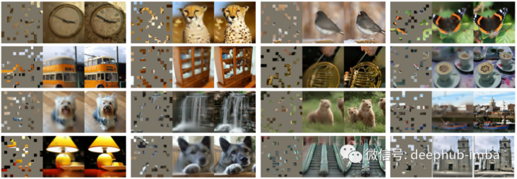
ImageNet validates the sample results of the image. From left to right: masking image, reconstructed image, real image. The masking rate is 80%.
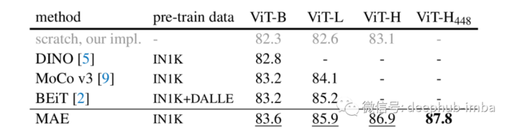
MAE also performs well in fine-tuning downstream tasks, such as image classification on ImageNet-1K dataset. Compared with the supervised method, when using MAE pre training for training, Vit large actually performed better than the baseline used.
The paper also includes the benchmark results of transfer learning experiments for downstream tasks and various ablation studies. If you are interested, you can look at the original paper.
discuss
If you are familiar with BERT, you may notice the similarities between the methods of BERT and MAE. In the pre training of BERT, we mask some texts, and the task of the model is to predict them. In addition, since we are now using a Transformer based architecture, it is not inappropriate to say that this method is visually equivalent to BERT.
But the paper says this method was earlier than BERT. For example, past attempts at image self-monitoring used stacked denoising self encoders and image restoration as pretext tasks. MAE itself also uses an automatic encoder as a model and a pretext task similar to image restoration.
If so, what makes MAE work better than previous models? I think the key is the ViT architecture. In their paper, the author mentioned that convolutional neural networks have problems in integrating "indicators" such as mask marking and location embedding, and ViT solves this architecture gap. If so, we will see another idea developed in natural language processing successfully implemented in computer vision. In the past, it was the attention mechanism, and then the concept of Transformer was borrowed into computer vision in the form of Vision Transformers. Now it is the whole BERT pre training process.
conclusion
I'm excited about what self-monitoring vision must provide in the future. In view of the success of BERT in natural language processing, mask modeling methods such as MAE will be beneficial to computer vision. Image data is easy to obtain, but marking them can be time-consuming. In this way, people can extend the pre training process by managing a much larger data set than ImageNet without worrying about tags. The potential is unlimited. Whether we will witness another revival of computer vision can only be proved by time.
quote
- Jacob Devlin, Ming-Wei Chang, Kenton Lee, and Kristina Toutanova. BERT: Pretraining of deep bidirectional transformers for language understanding. In NAACL, 2019.
- Kaiming He, Xinlei Chen, Saining Xie, Yanghao Li, Piotr Dollár, and Ross Girshick. Masked autoencoders are scalable vision learners. arXiv:2111.06377, 2021.
- Alexey Dosovitskiy, Lucas Beyer, Alexander Kolesnikov, Dirk Weissenborn, Xiaohua Zhai, Thomas Unterthiner, Mostafa Dehghani, Matthias Minderer, Georg Heigold, Sylvain Gelly, Jakob Uszkoreit, and Neil Houlsby. An image is worth 16x16 words: Transformers for image recognition at scale. In ICLR, 2021.
By Stephen Lau