1, Introduction to UAV
0 Introduction
With the development of modern technology, there are more and more types of aircraft, and their applications are becoming more and more specific and perfect, such as Dajiang PS-X625 UAV specially used for plant protection, Baoji Xingyi aviation technology X8 UAV used for street view shooting and monitoring patrol, and white shark MIX underwater UAV used for underwater rescue, The performance of aircraft is mainly determined by the internal flight control system and external path planning. As far as the path problem is concerned, only relying on the remote controller in the operator's hand to control the UAV to perform the corresponding work during the specific implementation of the task may put forward high requirements for the operator's psychology and technology. In order to avoid personal operation errors and the risk of aircraft damage, one way to solve the problem is to plan the flight path of the aircraft.
These changes, such as the measurement accuracy of aircraft, the reasonable planning of track path, the stability and safety of aircraft, have higher and higher requirements for the integrated control system of aircraft. UAV route planning is to design the optimal route to ensure that UAV can complete a specific flight mission and avoid various obstacles and threat areas in the process of completing the mission.
1 common track planning algorithms
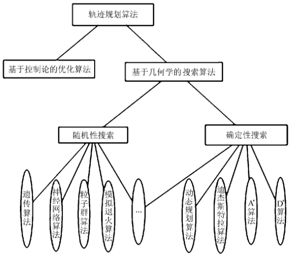
Figure 1 common path planning algorithms
This paper mainly studies the path planning of UAV in the cruise phase. Assuming that the UAV maintains the same altitude and speed in flight, the path planning becomes A two-dimensional plane planning problem. In the track planning algorithm, A algorithm is simple and easy to implement. Based on the improved A algorithm, A new and easy to understand UAV track planning method based on the improved A algorithm is proposed. The traditional A algorithm rasterizes the planning area, and the node expansion is limited to the intersection of grid lines. There are often two motion directions with A certain angle between the intersection and intersection of grid lines. Infinitely enlarge and refine the two paths with angles, and then use the corresponding path planning points on the two segments as the tangent points to find the center of the corresponding inscribed circle, and then make an arc, calculate the center angle of the arc between the corresponding two tangent points, and calculate the length of the arc according to the following formula

Where: R - radius of inscribed circle;
α——— The center angle corresponding to the arc between tangent points.
2, Introduction to particle filter algorithm
Particle filter is a Bayesian suboptimal estimation algorithm. It gets rid of the restriction that the random quantity must meet the Gaussian distribution when solving the nonlinear filtering problem, and solves the problem of lack of particle samples to a certain extent. Therefore, the algorithm has been successfully applied in many fields in recent years. However, the problem of particle degradation in particle filter seriously limits the development of its basic methods. See particle filter for details MCMC improved particle filter algorithm and its application in target tracking
3, Partial source code
% Function Description: ekf,ukf,pf,improvement pf UAV track prediction comparison program based on Algorithm
function main
% Because this program involves too many random numbers, let the random numbers remain unchanged every time
rand('seed',3);
randn('seed',6);
% error('The following parameters T Please refer to the value setting in the book and delete this line of code')
n = 9;
T = 50;
Q= [1 0 0 0 0 0 0 0 0; % Process noise covariance matrix
0 1 0 0 0 0 0 0 0;
0 0 1 0 0 0 0 0 0;
0 0 0 0.01 0 0 0 0 0;
0 0 0 0 0.01 0 0 0 0;
0 0 0 0 0 0.01 0 0 0;
0 0 0 0 0 0 0.0001 0 0;
0 0 0 0 0 0 0 0.0001 0;
0 0 0 0 0 0 0 0 0.0001];
R = [5000 0 0; % Observation noise covariance matrix
0 0.01^2 0 % The deviation of observation value of angle shall not be too large
0 0 0.01^2];
% System initialization
X = zeros(9,T); % True value
Z = zeros(3,T);
% Real state initialization
%X(:,1)=[1000;5000;200;10;50;10;2;-4;2]+sqrtm(Q)*randn(n,1);
X(:,1)=[100;500;20;10;50;10;2;-4;2]+sqrtm(Q)*randn(n,1);
state0 = X(:,1);
x0=0;
y0=0;
z0=0;
Station=[x0;y0;z0]; % Location of observation station
P0 =[100 0 0 0 0 0 0 0 0; % Covariance initialization
0 100 0 0 0 0 0 0 0;
0 0 100 0 0 0 0 0 0;
0 0 0 1 0 0 0 0 0;
0 0 0 0 1 0 0 0 0;
0 0 0 0 0 1 0 0 0;
0 0 0 0 0 0 0.1 0 0;
0 0 0 0 0 0 0 0.1 0
0 0 0 0 0 0 0 0 0.1];
%%%%%%%%%%%%% EKF filtering algorithm %%%%%%%%%%%%
Qekf = Q; % EKF Process noise variance
Rekf = R; % EKF Process noise variance
Xekf=zeros(9,T); % Filter state
Xekf(:,1)=X(:,1); % EKF Filter initialization
Pekf = P0; % covariance
Tekf=zeros(1,T); % Algorithm time consumption for recording a sampling period
%%%%%%%%%%%%% UKF filtering algorithm %%%%%%%%%%%%
Qukf = Q; % UKF Process noise variance
Rukf = R; % UKF Observation noise variance
Xukf=zeros(9,T); % Filter state
Xukf(:,1)=X(:,1); % UKF Filter initialization
Pukf = P0; % covariance
Tukf=zeros(1,T); % Algorithm time consumption for recording a sampling period
%%%%%%%%%%%%% PF filtering algorithm %%%%%%%%%%%%
N = 200; % Particle number
Xpf=zeros(n,T); % Filter state
Xpf(:,1)=X(:,1); % PF Filter initialization
Xpfset=ones(n,N); % Particle collection initialization
for j=1:N % Particle set initialization
Xpfset(:,j)=state0; % All initialized to x0,Each particle has equal values
end
Tpf=zeros(1,T); % Algorithm time consumption for recording a sampling period
%%%%%%%%%%%%% PF2 filtering algorithm %%%%%%%%%%%%
N2 = 200; % Particle number
R2 = [5000 0 0; % Observation noise covariance matrix
0 0.01^2 0 % The deviation of observation value of angle shall not be too large
0 0 0.01^2];
Xpf2=zeros(n,T); % Filter state
Xpf2(:,1)=X(:,1); % PF Filter initialization
Xpf2set=ones(n,N2); % Particle collection initialization
for j=1:N2 % Particle set initialization
Xpf2set(:,j)=state0; % All initialized to x0,Each particle has equal values
end
%%%%%%%%%%%%% PF3 filtering algorithm %%%%%%%%%%%%
N3 = 400; % Particle number
R3 = [5000 0 0; % Observation noise covariance matrix
0 0.01^2 0 % The deviation of observation value of angle shall not be too large
0 0 0.01^2];
Xpf3=zeros(n,T); % Filter state
Xpf3(:,1)=X(:,1); % PF Filter initialization
Xpf3set=ones(n,N3); % Particle collection initialization
for j=1:N3 % Particle set initialization
Xpf3set(:,j)=state0; % All initialized to x0,Each particle has equal values
end
Rekf2 = R2;
Xepf2=zeros(9,T); % Filter state
Xepf2(:,1)=X(:,1); % EPF Filter initialization
Xepf2set=ones(n,N2); % For initialization of particle set, it needs to be defined as a three-dimensional array, or, for simplicity, it needs to be defined as a one-time array(9xN)A two-dimensional array representing all particles in the current state
for j=1:N2 % Particle set initialization
Xepf2set(:,j)=state0; % All initialized to state0,Each particle has equal values
end
Pepf2 = P0*ones(n,n*N2);% Here, the covariance of each particle needs to be defined as a 3-dimensional array, or for simplicity, it needs to be defined as a 9 x(9xN)Two dimensional array of
%%%%%%%%%%%%% EPF3 filtering algorithm %%%%%%%%%%%%
Rekf3 = R3;
Xepf3=zeros(9,T); % Filter state
Xepf3(:,1)=X(:,1); % EPF Filter initialization
Xepf3set=ones(n,N3); % For initialization of particle set, it needs to be defined as a three-dimensional array, or, for simplicity, it needs to be defined as a one-time array(9xN)A two-dimensional array representing all particles in the current state
for j=1:N3 % Particle set initialization
Xepf3set(:,j)=state0; % All initialized to state0,Each particle has equal values
end
Pepf3 = P0*ones(n,n*N3);% Here, the covariance of each particle needs to be defined as a 3-dimensional array, or for simplicity, it needs to be defined as a 9 x(9xN)Two dimensional array of
%%%%%%%%%%%%% UPF filtering algorithm %%%%%%%%%%%%
Xupf=zeros(n,T); % Filter state
Xupf(:,1)=X(:,1); % UPF Filter initialization
Xupfset=ones(n,N); % Particle collection initialization
for j=1:N % Particle set initialization
Xupfset(:,j)=state0; % All initialized to state0,Each particle has equal values
end
Pupf = P0*ones(n,n*N); % Covariance of each particle
Tupf=zeros(1,T); % Algorithm time consumption for recording a sampling period
Xmupf = zeros(n,T); % Filter state
Tmupf = zeros(1,T);
%%%%%%%%%%%%%%%%%%%%%% Simulation system operation %%%%%%%%%%%%%%%%%%%%%%%%%
for t=2:T
% Simulate system status and run next step
[y1,y2,y3,y4,y5,y6,y7,y8,y9] = feval('ffun',X(:,t-1));
X(:,t)= [y1,y2,y3,y4,y5,y6,y7,y8,y9]'+ sqrtm(Q) * randn(n,1); % Generate actual state value
end
% Simulate the target movement process, and the observation station observes the target to obtain distance data
for t=1:T
[dd,alpha,beta]=feval('hfun',X(:,t),Station);
Z(:,t)= [dd,alpha,beta]'+sqrtm(R)*randn(3,1);
end
[Xepf(:,t),Xepfset,Pepf,Neffepf]=epf(Xepfset,Z(:,t),n,Pepf,N,R,Qekf,Rekf,Station); % Done
Tepf(t)=toc;
sum_epf = sum_epf + Neffepf;
% call EPF2 algorithm
[Xepf2(:,t),Xepf2set,Pepf2,Neffepf]=epf(Xepf2set,Z(:,t),n,Pepf2,N2,R2,Qekf,Rekf2,Station); % Done
% call EPF3 algorithm
[Xepf3(:,t),Xepf3set,Pepf3,Neffepf]=epf(Xepf3set,Z(:,t),n,Pepf3,N3,R3,Qekf,Rekf3,Station); % Done
% call UPF algorithm
%tic
%[Xupf(:,t),Xupfset,Pupf]=upf(Xupfset,Z(:,t),n,Pupf,N,R,Qukf,Rukf,Station); % 1
%Tupf(t)=toc;
end
%%%%%%%%%%%%%%%%%%%%%% Data analysis %%%%%%%%%%%%%%%%%%%%%%%%%
% assume
for i = 1:T
Xupf(:,i) = X(:,i) + 2 * sin(t);
end
% RMS Deviation comparison diagram
EKFrms = zeros(1,T);
UKFrms = zeros(1,T);
PFrms = zeros(1,T);
EPFrms = zeros(1,T);
PF2rms = zeros(1,T);
EPF2rms = zeros(1,T);
PF3rms = zeros(1,T);
EPF3rms = zeros(1,T);
UPFrms = zeros(1,T);
end
% X axis RMS Deviation comparison diagram
EKFXrms = zeros(1,T);
UKFXrms = zeros(1,T);
PFXrms = zeros(1,T);
EPFXrms = zeros(1,T);
% X axis RMS Deviation comparison diagram
EKFYrms = zeros(1,T);
UKFYrms = zeros(1,T);
PFYrms = zeros(1,T);
EPFYrms = zeros(1,T);
% Z axis RMS Deviation comparison diagram
EKFZrms = zeros(1,T);
UKFZrms = zeros(1,T);
PFZrms = zeros(1,T);
EPFZrms = zeros(1,T);
for t=1:T
EKFXrms(1,t)=abs(X(1,t)-Xekf(1,t));
UKFXrms(1,t)=abs(X(1,t)-Xukf(1,t));
PFXrms(1,t)=abs(X(1,t)-Xpf(1,t));
EPFXrms(1,t)=abs(X(1,t)-Xepf(1,t));
EKFYrms(1,t)=abs(X(2,t)-Xekf(2,t));
UKFYrms(1,t)=abs(X(2,t)-Xukf(2,t));
PFYrms(1,t)=abs(X(2,t)-Xpf(2,t));
EPFYrms(1,t)=abs(X(2,t)-Xepf(2,t));
EKFZrms(1,t)=abs(X(3,t)-Xekf(3,t));
UKFZrms(1,t)=abs(X(3,t)-Xukf(3,t));
PFZrms(1,t)=abs(X(3,t)-Xpf(3,t));
EPFZrms(1,t)=abs(X(3,t)-Xepf(3,t));
end
% Drawing, three-dimensional trajectory
NodePostion = [100,800,100;
200,800,900;
0,0,0];
figure
t=1:T;
hold on;
box on;
grid on;
for i=1:3
p8=plot3(NodePostion(1,i),NodePostion(2,i),NodePostion(3,i),'ro','MarkerFaceColor','b');
text(NodePostion(1,i)+0.5,NodePostion(2,i)+0.5,NodePostion(3,i)+1,
figure
hold on;
box on;
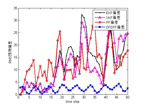
p1=plot(1:T,EKFrms,'-k.','lineWidth',2);
p2=plot(1:T,UKFrms,'-m^','lineWidth',2);
p3=plot(1:T,PFrms,'-ro','lineWidth',2);
%p4=plot(1:T,EPFrms,'-g*','lineWidth',2);
p5=plot(1:T,UPFrms,'-bp','lineWidth',2);
legend([p1,p2,p3,p5],'EKF deviation','UKF deviation','PF deviation','DFEPF deviation');
xlabel('time step');
ylabel('RMS Prediction deviation');
figure;
hold on;
box on;
p1=plot(1:T,PFrms,'-k.','lineWidth',2);
p2=plot(1:T,EPFrms,'-m^','lineWidth',2);
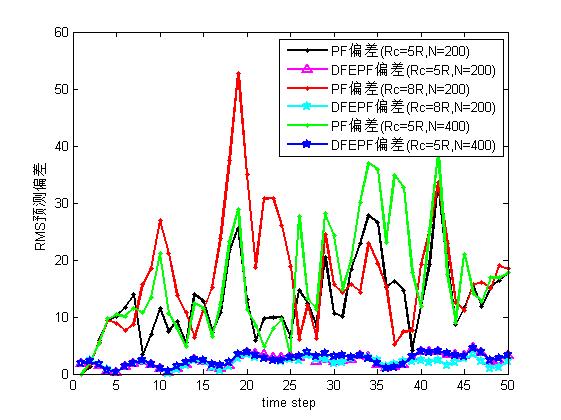
p3=plot(1:T,PF2rms,'-r.','lineWidth',2);
p4=plot(1:T,EPF2rms,'-cp','lineWidth',2);
p5=plot(1:T,PF3rms,'-g.','lineWidth',2);
p6=plot(1:T,EPF3rms,'-bp','lineWidth',2);
legend([p1,p2,p3,p4,p5,p6],'PF deviation(Rc=5R,N=200)','DFEPF deviation(Rc=5R,N=200)','PF deviation(Rc=8R,N=200)','DFEPF deviation(Rc=8R,N=200)','PF deviation(Rc=5R,N=400)','DFEPF deviation(Rc=5R,N=400)');
xlabel('time step');
ylabel('RMS Prediction deviation');
figure;
hold on;
box on;
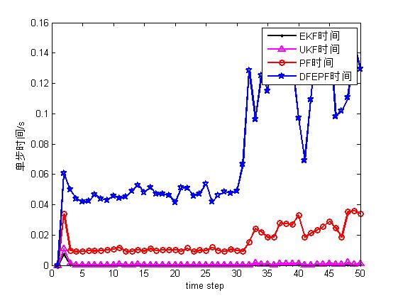
p1=plot(1:T,Tekf,'-k.','lineWidth',2);
p2=plot(1:T,Tukf,'-m^','lineWidth',2);
p3=plot(1:T,Tpf,'-ro','lineWidth',2);
p4=plot(1:T,Tepf,'-bp','lineWidth',2);
legend([p1,p2,p3,p4],'EKF time','UKF time','PF time','DFEPF time');
xlabel('time step');
ylabel('Single step time/s');
%%%%%%%%%%%%%%%%%%%%%%%%%%%%%%%%%%%%%%%%%%%%%%%%%%%%%%%%%%%%%%%%%%%%%%%%%%
% Draw a different one Q,R Different results are obtained
% Draw another deviation curve
4, Operation results
5, matlab version and references
1 matlab version
2014a
2 references
[1] Steamed stuffed bun Yang, Yu Jizhou, Yang Shan Intelligent optimization algorithm and its MATLAB example (2nd Edition) [M]. Electronic Industry Press, 2016
[2] Zhang Yan, Wu Shuigen MATLAB optimization algorithm source code [M] Tsinghua University Press, 2017
[3] Wu Xi, Luo Jinbiao, Gu Xiaoqun, Zeng Qing Optimization algorithm of UAV 3D track planning based on Improved PSO [J] Journal of ordnance and equipment engineering 2021,42(08)
[4] Deng ye, Jiang Xiangju Four rotor UAV path planning algorithm based on improved artificial potential field method [J] Sensors and microsystems 2021,40(07)
[5] Ma Yunhong, Zhang Heng, Qi Lerong, he Jianliang 3D UAV path planning based on improved A * algorithm [J] Electro optic and control 2019,26(10)
[6] Jiao Yang Research on UAV 3D path planning based on improved ant colony algorithm [J] Ship electronic engineering 2019,39(03)