preface

The pioneering work of the VIT model is to use a pure transformer structure, as shown in the title of the paper: AN IMAGE IS WORTH 16X16 WORDS, which embeds the pictures into a series of sequence s, and realizes the effect comparable to the SOTA model in CNN through multiple encoder structures and head s.

Image classification task ranking

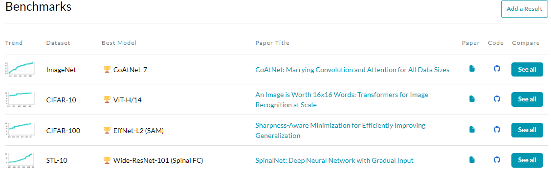
CNN has dominated the major image task lists for a long time. Before, it was sometimes thought that the CNN structure was the best structure, but it seems that the recent data have been shamed. Why do you say so? Among the major image task rankings of paperwithcode (such as segmentation and detection), the transformer based model has occupied the top or even the top ten of the major rankings. The real data are here. We can't help asking: are we going to bid farewell to the CNN era? Here is just a question, and it's also the editor's own question.
This article is an analysis of VIT. Now we officially begin to introduce the vit model.
As transformer challenges RNN in various nlp fields, and with the release of BERT and GPT models, transformer shows its excellent generalization ability of downstream tasks and unsatisfied "appetite" under large-scale data in large-scale models. Slowly, CV field also begins to be noticed.

VIT model architecture

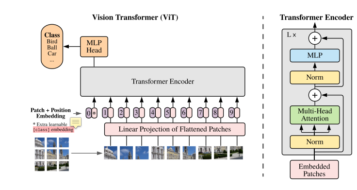
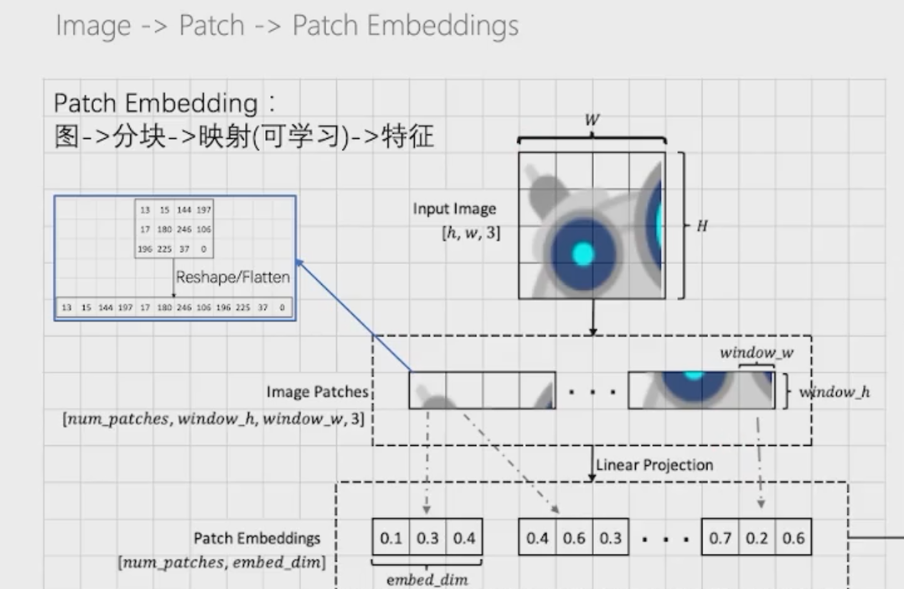
As shown in the figure, I believe friends with transformer learning experience can see the architecture of the author's model at a glance. This figure is simple and easy to understand. VIT patch embedding the picture, That is, divide the picture into multiple blocks (patch), and then expand each patch into a sequence sequence sequence through embedding. At the same time, in order to carry out the classification task, the author introduces an additional class token, that is, the vector of the 0 position of the input sequence, as the classification task. The HEAD carries out the type prediction by a multi HEAD attention and mlp layer. The overall structure is simple and clear, making people feel like a spring breeze.

I abstract

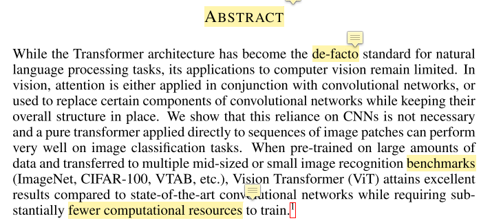
The author first introduces the achievements of attention mechanism in the field of nlp, and then there are some hybrid models based on attention mechanism and convolution. The author abandons the traditional CNN structure and proposes a model based on pure transformer. In terms of experiments, the author uses the data sets trained on large data sets and migrated to small and medium-sized data sets for effect verification. Its performance can be comparable to the current SOTA convolution network model, and requires less computational power (here refers to 2500 days tpu v3, which is enough to see the author's strong financial resources)

II introduction

2.1 this part mainly introduces

1. The current situation of transformer in nlp field explains why it can dominate nlp field in recent papers, that is, its advantages
2. The application status of transformer in the image field still has the image bias assumption, and it is difficult to accelerate on the modern gpu. This leads to the author's work, that is, motivation. It also explains the problem that the author wants to solve: hybrid structure can not outperform all cnn structure in cv, In other words, the author wants to try that the pure transformer structure can show better results than VNN in visual tasks.
3. This paper introduces the structural characteristics proposed by the author, puts forward and solves the important problems in the experimental process, that is, under the same data set, the performance of VIT is always lower than that of CNN (as shown in the following English summary). Finally, the author shows the excellent performance of his model.

When pre-trained on the public ImageNet-21k dataset or the in-house JFT-300M dataset, ViT 
approaches or beats state of the art on multiple image recognition benchmarks. In particular,
the best model reaches the accuracy of 88.55% on ImageNet, 90.72% on ImageNet-ReaL, 94.55%
 on CIFAR-100, and 77.63% on the VTAB suite of 19 tasks.

2.2 inductive biases

In his article, the author mentioned inductive bias many times, that is, convolution. In the traditional convolution, we introduce two assumptions, that is, a priori:

1. Translation invariance: when the trained convolution kernel faces the same picture, the characteristic pictures expressed or generated are similar, or it is only interested in something in the picture.
2. Local correlation: during the sliding process of convolution kernel, two adjacent generated pixels are related due to weight sharing.
   By introducing the above two assumptions, we artificially bring a priori knowledge to the model. Therefore, the author in order to remove this artificial hypothesis. In another view, in order to compensate for the performance degradation caused by transformer's removal of inductive bias, the author adds a large number of training data to compensate. In fact, it is to learn these two inductive biases with more data. There are different opinions here. The author himself brings us another way of thinking.

2.3 related work

Remember a sentence in Mu Shen's class:
A lot of related work is written here, which will not make your work seem very few and simple, but will make your paper easier to understand.

2.3. 1 brief introduction

1. This paper first describes the latest progress of transformer in the nlp field, and then puts forward the related work and problems of transformer in the image field: for example, the computational disaster caused by expanding the image directly according to the pixel size, the local attention mechanism, the spark transformer, or only paying attention to the pixels of a single reference axis, but these methods all have a problem, It is difficult to apply to modern gpu because its preprocessing steps are too cumbersome. What the author asks is a brief introduction.

2. The most similar related work is proposed and compared: first, the patch size proposed by predecessors is too small, so it can only be applied to small resolution images; second, the author does pre training on large data sets to achieve the effect of SOTA.

3. Write another idea: hybrid mathod, DETR is to take resnet as the backbone and feature graph as the input sequence.

4. Write about some recent developments: iGPT.

Finally, the author analyzes the effect of large data sets rather than standard Imagenet data sets on model training, and gives some performance of cnn under different scales of data sets.
In conclusion, the author analyzes the reason why this pure transformer structure is proposed. On the other hand, the igpt, which is born due to the influence of bert, is given. Finally, the important role of large data sets in model performance is explained.

III Method & recurrence

3.1 image processing

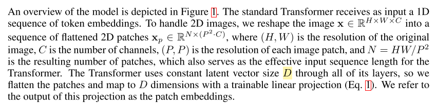
Step 1: the original input picture is of (H, W, C) size. First, divide it into square blocks of P size:

N=H∗W/(P∗P)

Step 2: N is the number of segmented blocks, which is also the number of patches. Flatten the picture, that is, expand it into 2Dpatch, N P ² * C-size patch.

Step 3: add position vector and class token vector, where position vector is a learnable parameter.

3.1. 1 replication (based on the paddlepaddle framework)

patch embedding

#patch embedding process
class PatchEmbedding(nn.Layer):
    def __init__(self, image_size=224, patch_size=16, in_channels=3, embed_dim=768, dropout=0.):
        super().__init__()
        self.embed_dim = embed_dim
        n_patches = (image_size // patch_size) * (image_size // patch_size)
        self.patch_embedding = nn.Conv2D(in_channels=in_channels,
                                         out_channels=embed_dim,
                                         kernel_size=patch_size,
                                         stride=patch_size)
        self.dropout = nn.Dropout(dropout)

        # TODO: add class token
        self.class_token = paddle.create_parameter(#Here, a learnable class token vector is added for downstream tasks such as classification
            shape = [1, 1, embed_dim],
            dtype = 'float32',
            default_initializer = nn.initializer.Constant(0.),
        )
        # TODO: add position embedding
        self.position_embedding = paddle.create_parameter(#Add a learnable position vector
            shape = [1, n_patches + 1, embed_dim],
            dtype='float32',
            default_initializer=nn.initializer.TruncatedNormal(std=.02)
        )

    def forward(self, x):
        # [n, c, h, w] original picture size: each batch contains n pictures, each of which is h * w * c
        class_token = self.class_token.expand([x.shape[0], 1, self.embed_dim])#Since the size of the input picture is not fixed, expand is used
         #Here, the image is segmented and convolution is used to achieve a similar effect when stripe = kernel_ When the size is, the patch is generated
        x = self.patch_embedding(x)
        x = x.flatten(2)
        x = x.transpose([0, 2, 1])
        x = paddle.concat([class_token, x], axis=1)
        #Add position vector
        x = x + self.position_embedding

        return x

After completing the previous paragraph, we have finished encoding the picture. So far, we can input the returned tensor into the attention layer for calculation.

attention layer

In this paragraph, we mainly reproduce the part of attention:

#In the attention section, enter the patch embedding returned from the previous code into the attention layer
class Attention(nn.Layer):
    """multi-head self attention"""
    def __init__(self, embed_dim, num_heads, qkv_bias=True, dropout=0., attention_dropout=0.):
        super().__init__()
        self.num_heads = num_heads
        self.head_dim = int(embed_dim / num_heads)#Number of calculation heads
        self.all_head_dim = self.head_dim * num_heads
        self.scales = self.head_dim ** -0.5#Calculate the scaling factor, which is dk under the root sign
		#qkv initialization
        self.qkv = nn.Linear(embed_dim,
                             self.all_head_dim * 3,
                             bias_attr=False if qkv_bias is True else None
                             )
		#The linear layer here mainly serves as the final output of mlp
        self.proj = nn.Linear(embed_dim, embed_dim)

        self.dropout = nn.Dropout(dropout)
        self.attention_dropout = nn.Dropout(attention_dropout)
        self.softmax = nn.Softmax(axis=-1)

    def transpose_multihead(self, x):#This function converts x to the desired format
        # x: [N, num_patches, all_head_dim] -> [N, n_heads, num_patches, head_dim]
        new_shape = x.shape[:-1] + [self.num_heads, self.head_dim]
        x = x.reshape(new_shape)
        x = x.transpose([0, 2, 1, 3])
        return x

    def forward(self, x):
        # TODO
        B, N, _ = x.shape
        qkv = self.qkv(x).chunk(3, -1)
        q, k, v = map(self.transpose_multihead, qkv)
        atten = paddle.matmul(q, k, transpose_y = True)#Computational attention
        atten = atten * self.scales#Scaling
        atten = self.softmax(atten)
        out = paddle.matmul(atten, v)#Attention matrix calculation
        out = out.transpose([0, 2, 1, 3])
        out = out.reshape([B, N, -1])
        #out:[b, n, num_heads * head_dim]
        out = self.proj(out)
        return out

class ViT(nn.Layer):
    def __init__(self):
        super().__init__()
        self.patch_embed = PatchEmbedding(224, 7, 3, 16)
        layer_list = [EncoderLayer(16) for i in range(5)]#stack is a five layer encoder, and the size of each embedding dimension is 16
        self.encoders = nn.LayerList(layer_list)
        self.head = nn.Linear(16, 10)#Here is the classification layer. The input is 16 dimensions and the output is 10 dimensions, that is, it is divided into ten categories
        self.avgpool = nn.AdaptiveAvgPool1D(1)#Here is the 1-dimensional average pool, which is used to average all patch outputs for classification

    def forward(self, x):
        x = self.patch_embed(x) # [n, h*w, c]: 4, 1024, 16
        for encoder in self.encoders:
            x = encoder(x)#Superposition of multiple encoder s
        # avg
        x = x.transpose([0, 2, 1])#Transpose [n, h * w, c] to [n, c, h * w]
        x = self.avgpool(x)#[n, c, 1]
        x = x.flatten(1)#[n*c], i.e. [16, 1]
        x = self.head(x)
        return x

To sum up, the forward structure reproduction from the patch embedding of the picture to the prediction of the final classification result is completed.

3.2 FINE-TUNING AND HIGHER RESOLUTION

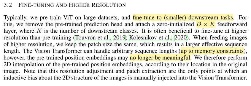
The author mentioned that if the VIT trained model is applied to downstream tasks, only the predicted HEAD header needs to be removed, Then connect a zero initialized forward prediction layer of D*K behind the VIT (D is the number of layers and K is the number of categories of downstream tasks) to realize the downstream tasks. At the same time, VIT can process sequences of any length, and the length of the sequence is limited by the patch size and memory (the patch will be temporarily put into memory for calculation), but if it becomes longer, the pre trained position code will be invalid and need to be retrained.
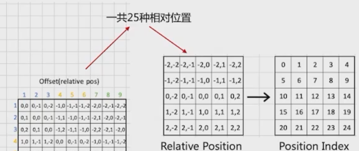
The author compares the similarities and differences between position coding 1D and 2D coding (as shown in the figure below). Through the comparison, the author does not find that there is a large performance difference between the two coding methods. At the same time, the author believes that 2D coding will introduce the problem of image inductive bias, which deviates from the original intention of the author to abandon inductive bias.

2D position coding

IV experiment

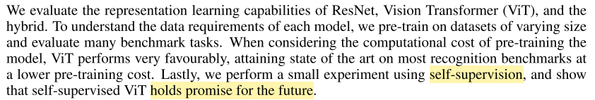
The pure convolution method represented by the author and ResNet and * * Hybrid (Hybrid model) * * performance comparison experiments are carried out. At the same time, in order to explain the demand for data volume of each model, the author trains it on different data sets and migrates it to different benchmark to verify the effect. Facts have proved that it achieves SOTA effect with lower pre training cost. The author also shows expectations for self-monitoring training.
The following are three models of different sizes designed by the author, with different scales set for their size and parameter size.

It can be seen that on the VIT-HUGE version, in imagenet as a benchmark, the author's model performance exceeds RESNET by more than one percentage point, and the number of days to be trained is also lower than 9.9k of RESNET.

The following figure shows the author's visual output in order to better understand the image processing mechanism within VIT.

The following figure is the result of the author's visualization of the learned position coding (the first 28 principal components are selected). The image shows that the position coding similarity of adjacent positions is higher.

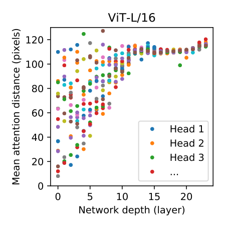
At the same time, the experiment shows that, as shown in the figure below, the deeper the layer, the farther the multi head's attention range to the overall situation, which is actually like cnn. The deeper the number of layers, the higher the abstraction degree of features, the larger the range of features can be seen, and the larger the receptive field.

Summary and evaluation

On the whole, the transformer proposed by the author has played a milestone in its contribution to the visual transformer. Many of the models proposed later for various downstream tasks are based on this structure.
In terms of leadership, although the author's structure has too high requirements for small target detection and training computing power, here, as when alexnet was put forward, any newly proposed revolutionary model must go through the process of putting forward - discovering problems - improving and perfecting, just like swin transformer, which recently occupied the top of the list, is patched on this basis.

The author mainly puts forward two points:
1. Compared with the previous model based on visual transformer, the author introduces patch to avoid the inductive bias caused by convolution and adds learnable image position coding.
2. The author proves the feasibility of VIT migrating to small data sets after training in large data sets, and can be comparable to SOTA's CNN structure.

At the same time, the author makes a prospect:
1. Downstream tasks: segmentation and detection can be further developed.
2. Exploration of self supervised pre training method.