Content of this article

1. introduce
2. AdaBoost
3. Gradient Boost
4. XGBoost
5. Histogram-Based Gradient Boost
6. LightBoost
7. CatBoost
8. summary

introduce

In ensemble learning, the goal is to train the model most successfully with a variety of learning algorithms. Bagging method is an integrated learning method, which applies multiple models to different sub samples of the same data set in parallel. Boosting is another method often used in practice. It is not built in parallel, but in order. The purpose is to train algorithms and models. The weak algorithm first trains the model, and then reorganizes the model according to the training results to make the model easier to learn. Then the modified model is sent to the next algorithm. The second algorithm is easier to learn than the first algorithm. This paper includes different enhancement methods, explains these methods from different angles, and makes simple tests.

AdaBoost

Adaptive lifting (Adaboost) is a widely used decision tree based method (Decision stump: Threshold isassigned and the Prediction is made by the threshold.) but this method is not blindly repeated in Adaboost. Multiple algorithms are established, which update their weights in turn and play their respective roles in making the most accurate estimation. The error rate of each algorithm is calculated. The weights are updated, so It is cited in the second algorithm. The second algorithm classifies the model, updates the weight like the first model, and transfers it to the third algorithm. These processes continue until n_ Number of estimators or error = 0. In this process, because the weights are updated by the previous algorithm and sent to other algorithms, the classification is easier and more successful. Let's explain this complex sequential algorithm process with an example:

Suppose there are two labels, red and blue. The first algorithm (weak classifier 1) separates the labels, and the result is that two blue samples and one red sample are misclassified. The weight of these wrong classifications increases, and the weight of correct classification decreases, which is sent to the next model for learning. In the new model, the deviation of incorrectly classified samples increases and the deviation of correctly classified samples decreases. The learning effects of the two models are better. The next steps repeat the same process. To sum up, strong classification occurs with the cooperation of weak classification. Because it is used for classification, it can also be used for regression by importing AdaBoost regressor.

Super parameter

base_estimators: a sequential improved algorithm class (default = DecisionTreeClassifier)

n_estimators: determine the maximum number of steps that the above process will take. (default = 50)

learning_rate: determines the amount of weight change. If the selection is too small, n_ The value of estimators must be very high. If it is chosen too large, it may never reach the optimal value. (default = 1)

import numpy as np
from time import time
from sklearn.datasets import make_classification 
from sklearn.model_selection import cross_val_score,train_test_split
from sklearn.model_selection import KFold

x,y = make_classification(n_samples=100000,n_features=30, n_informative=10, 
                          n_redundant=5,random_state=2021)

A dataset that will be used for all methods has been imported. Now let's implement Adaboost:

from sklearn.ensemble import AdaBoostClassifier

start_ada = time()
ada = AdaBoostClassifier()

kf=KFold(n_splits=5,shuffle=True,random_state=2021)
ada_score=cross_val_score(ada,x,y,cv=kf,n_jobs=-1)
print("ada", np.round(time()-start_ada,5),"sec")
print("acc", np.mean(ada_score).round(3))
print("***************************")

Gradient Boost

Adaboost improves itself by updating the weights using decision tree stumps (one node is divided into two leaves). Gradient lifting is another sequential method, which optimizes the loss by creating 8 to 32 leaves, which means that the tree is larger in gradient lifting (loss: like the residual in the linear model). (y_test-y_prediction) The sum of squares of losses is given by each data point, and the residual is given. Why use square? Because the value we are looking for is the deviation between the prediction and the actual results. The square of negative value will also act on the calculation of loss value. In short, the residual value is transferred to the next algorithm to make the residual value closer to 0, so as to minimize the loss value.

GB = GradientBoostingClassifier()

start_gb = time()
kf=KFold(n_splits=5,shuffle=True,random_state=2021)
GB_score=cross_val_score(GB,x,y,cv=kf,n_jobs=-1)
print("gb", np.round(time()-start_gb,5),"sec")
print("acc", np.mean(GB_score).round(3))
print("***************************")

In Adaboost, gradient enhancement can be used for regression by importing GradientBoostRegressor.

from sklearn.metrics import mean_squared_error
x_train, x_test, y_train, y_test = train_test_split(x, y,test_size=0.2,random_state=2021)
gbr = GradientBoostingRegressor(max_depth=5, n_estimators=150)
gbr.fit(x_train, y_train)
error_list = [mean_squared_error(y_test, y_pred) for y_pred in gbr.staged_predict(x_test)]

OUT
[0.22686585533221332,0.20713350861706786,0.1900682640534445,
 0.1761959477525979,0.16430532532798403,0.1540494010479854,
 0.14517117541343785,0.1375952312491854,0.130929810958826,
 0.12499605002264891,0.1193395594019215,0.11477096339545599,
 0.11067921343289967,0.10692446632551068,...................
 ...........................................................
 0.05488031632425609,0.05484366975329703,0.05480676108875857,
 0.054808073418709524,0.054740333154284,0.05460221966859833,
 0.05456647041868937,0.054489873127848434,0.054376259548495065,
 0.0542407250628274]

View Error_list, you can see that the loss value is decreasing at each step. [from 0.22 to 0.05]

XGBoost

XGBoost(Extreme Gradient Boosting) was developed by Tianqi Chen in 2014. It is the fastest before Gradient boost and is the preferred Boosting method. Because it contains hyperparameters, many adjustments can be made, such as regularizing hyperparameters to prevent over fitting.

Super parameter

booster [default = gbtree]
Decide to use the booster, which can be gbtree, gblinear or dart. Gbtree and dart use tree - based models, while gblinear uses linear functions

silent [default = 0]
Set to 0 to print operation information; Set to 1 silent mode, do not print

nthread [default = set to maximum possible number of threads]
For the number of threads running xgboost in parallel, the input parameter should be < = the number of CPU cores of the system. If it is not set, the algorithm will detect and set it to all the cores of the CPU
The following two parameters do not need to be set. Just use the default

num_pbuffer [xgboost is automatically set, no user setting is required]
The size of the prediction result cache is usually set to the number of training instances. This cache is used to store the prediction results of the last boosting operation.

num_feature [xgboost is automatically set, no user setting is required]
Use the dimension of the feature in boosting and set it as the maximum dimension of the feature

eta [default = 0.3, alias: learning_rate]
Reduce the step size in the update to prevent overfitting. After each boosting, new feature weights can be obtained directly, which can make the boosting more robust.
Range: [0,1]

gamma [default = 0, alias: min_split_loss]
When a node is split, it will split only when the value of the loss function decreases after splitting. Gamma specifies the minimum loss function drop value required for node splitting. The larger the value of this parameter, the more conservative the algorithm is. The value of this parameter is closely related to the loss function, so it needs to be adjusted.
Range: [0, ∞]

max_depth [default = 6]
This value is the maximum depth of the tree. This value is also used to avoid over fitting. max_ The greater the depth, the more specific and local samples the model will learn. Setting to 0 means there is no limit
Range: [0, ∞]

min_child_weight [default = 1]
Determine the minimum leaf node sample weight and. This parameter of XGBoost is the sum of the minimum sample weights, while the GBM parameter is the minimum total number of samples. This parameter is used to avoid over fitting. When its value is large, the model can avoid learning local special samples. However, if this value is too high, it will lead to under fitting. This parameter needs to be adjusted using CV
Range: [0, ∞]

subsample [default = 1]
This parameter controls the proportion of random sampling for each tree. Reducing the value of this parameter will make the algorithm more conservative and avoid over fitting. However, if this value is set too small, it may result in under fitting. Typical value: 0.5-1, 0.5 represents average sampling to prevent over fitting
Range: (0,1]

colsample_bytree [default = 1]
It is used to control the proportion of the number of columns sampled randomly per tree (each column is a feature). Typical value: 0.5-1
Range: (0,1]

colsample_bylevel [default = 1]
It is used to control the sampling proportion of the number of columns for each split of each level of the tree. Personally, I don't usually use this parameter because the subsample parameter

colsample_ The bytree parameter can do the same. However, if you are interested, you can mine this parameter for more use.
Range: (0,1]

Lambda [default = 1, alias: reg_lambda]
L2 regularization term of weight. (similar to ridge expression). This parameter is used to control the regularization part of XGBoost. Although most data scientists rarely use this parameter, it can be more useful in reducing over fitting

Alpha [default = 0, alias: reg_alpha]
L1 regularization term of weight. (similar to lasso region). It can be applied in the case of high dimensions to make the algorithm faster.

scale_pos_weight [default = 1]
When all kinds of samples are very unbalanced, setting this parameter to a positive value can make the algorithm converge faster. It can usually be set as the ratio of the number of negative samples to the number of positive samples.

from xgboost import XGBClassifier

xgb = XGBClassifier()

start_xgb = time()
kf=KFold(n_splits=5,shuffle=True,random_state=2021)
xgb_score=cross_val_score(xgb,x,y,cv=kf,n_jobs=-1)
print("xgboost", np.round(time()-start_xgb,5))
print("acc", np.mean(xgb_score).round(3))
print("***************************")

Histogram-Based Gradient Boost

Using binning(discretizing) to group data is a data preprocessing method, which has been explained here. For example, when the "age" column is given, it is a very effective method to divide these data into three groups: 30-40, 40-50 and 50-60, and then convert them into numerical data. When this method is suitable for decision tree, it can speed up the algorithm by reducing the number of features. This method can also be used as an integration for building each tree by grouping it with histogram.

from sklearn.experimental import enable_hist_gradient_boosting
from sklearn.ensemble import HistGradientBoostingClassifier

HGB = HistGradientBoostingClassifier()

start_hgb = time()
kf=KFold(n_splits=5,shuffle=True,random_state=2021)
HGB_score=cross_val_score(HGB,x,y,cv=kf,n_jobs=-1)
print("hist", np.round(time()-start_hgb,5),"sec")
print("acc", np.mean(HGB_score).round(3))
print("***************************")

LightBoost

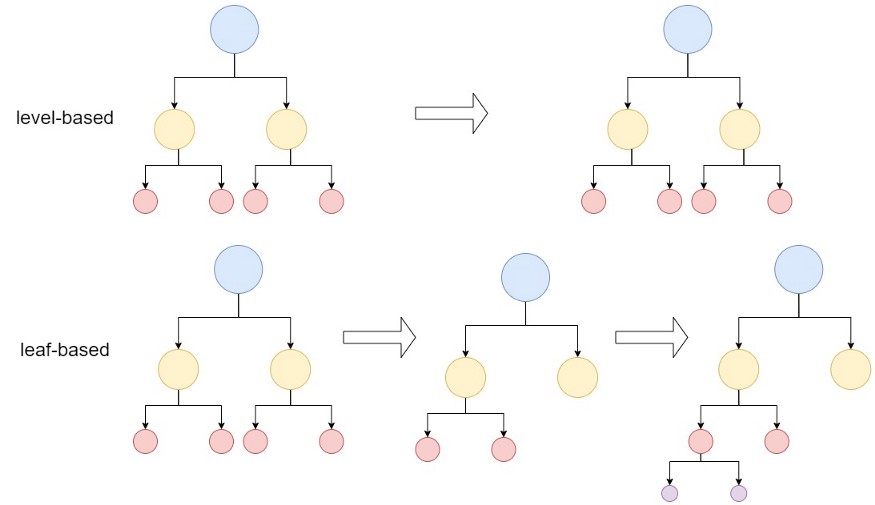
LGBM (Light Gradient Boosting Machine) is a gradient enhancement method based on decision tree first released by Microsoft in 2017. It is another gradient enhancement method preferred by users. The key difference from other methods is that it splits the tree based on leaves, That is, it can be detected and calculated by key points (other lifting algorithms are based on depth or level). Since LGBM is leaf based, as shown in Figure 2, LGBM is a very effective method to reduce errors and improve accuracy and speed. However, it does not support string type data. Special algorithms need to be used to split classification data, because integer values must be entered (such as an index) instead of the string name of the column.

from lightgbm import LGBMClassifier

lgbm = LGBMClassifier()

start_lgbm = time()
kf=KFold(n_splits=5,shuffle=True,random_state=2021)
lgbm_score=cross_val_score(lgbm,x,y,cv=kf,n_jobs=-1)
print("lgbm", np.round(time()-start_lgbm,5))
print("acc", np.mean(lgbm_score).round(3))
print("***************************")

CatBoost

Catboost was developed by Yandex in 2017. Because it uses one hot encoding to convert all classification features to numeric values, the name comes from category boosting. It automatically converts the string into an index value. It also handles missing values. And it's much faster than XGBoost. Unlike other boosting methods, catboost is distinguished from symmetric tree, which uses the same splitting in nodes at each level.

XGBoost and LGBM calculate the residual of each data point and train the model to obtain the residual target value. It repeats this operation for the number of iterations to train and reduce the residuals to achieve the goal. Since this method is applicable to each data point, it may be weak in generalization and lead to over fitting.

Catboost also calculates the residual of each data point and uses the model trained by other data. In this way, each data point gets different residual data. These data are evaluated as targets, and the training times of the general model are as many as the number of iterations. Since many models will be implemented by definition, this computational complexity seems very expensive and takes too much time. However, catboost can be completed in a shorter time through orderly promotion. For example, catboost does not start from the beginning of the residual calculated for each data point (n+1)th. Russia and Japan calculate (n+2) data points, apply (n+1) data points, and so on

Super parameter

l2_leaf_reg: L2 regularization term of loss function.

learning_rate: learning rate. Reduce learning in the case of over fitting_ rate.

Depth: the depth of the tree. It is usually used between 6 and 10.

one_hot_max_size: all classification features are coded with a unique heat code, and several different values are less than or equal to the given parameter values

grow_policy: determines the construction type of the tree. You can use SymmetricTree, Depthwise, or Lossguide.

from catboost import CatBoostClassifier

cat = CatBoostClassifier()

start_cat = time()
kf=KFold(n_splits=5,shuffle=True,random_state=2021)
cat_score=cross_val_score(cat,x,y,cv=kf,n_jobs=-1)
print("cat", np.round(time()-start_cat,5))
print("acc", np.mean(cat_score).round(3))
print("***************************")

summary

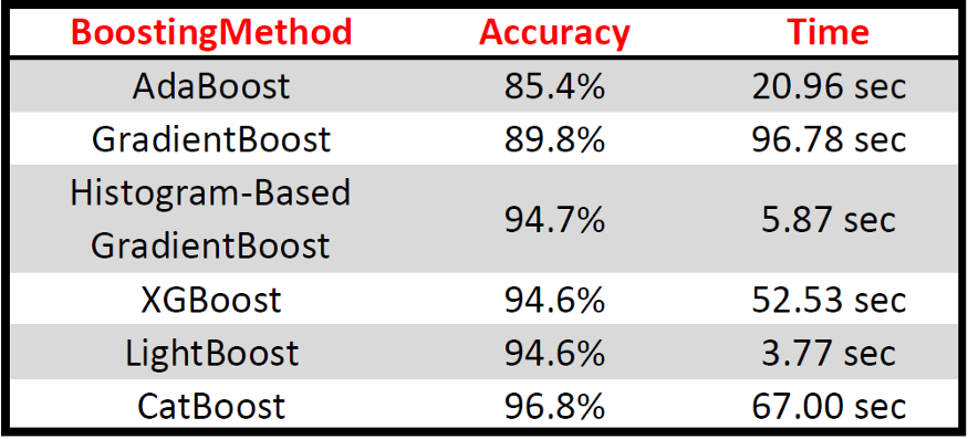
In this article, DecisionTree is used to deal with the promotion method, but other machine learning models can be easily implemented by changing the relevant super parameters. In addition, all boosting methods use base version (without adjusting any super parameters) to compare the performance of boosting methods. The code applied above is shown in the following table:

Author: Ibrahim Kovan