I. Introduction
1. Overview of basic principle of template matching
When comparing two images, the first basic problem we face is: when are the two images the same or similar, and how to measure the similarity of the two images? Of course, the general method is that when the gray values of all pixels of the two images are the same, we think such images are the same. This comparison method is feasible in some specific application fields, such as detecting the change of two consecutive frames in constant illumination environment and camera internal environment. Simply comparing the difference between pixels is not appropriate in most applications. Noise, quantization error, small illumination change, small translation or rotation will produce a large pixel difference when the pixels of the two images are simply different, but the two images are still the same when viewed by human eyes. Obviously, human perception can sense a wider range of similar content. Even when the difference of a single pixel is large, it can use such as structure and image content to identify the similarity of two images. Comparing images at the structural or semantic level is not only a difficult problem, but also an interesting research field.
Here we introduce a relatively simple image comparison method at the pixel level. That is, locate a given sub image - template image in a larger image, which is commonly referred to as template matching. This often happens, such as locating a specific object in an image scene, or tracking some specific patterns in an image sequence. The basic principle of template matching is very simple: in the image to be searched, move the template image, measure the difference between the sub image of the image to be searched and the template image at each position, and record its corresponding position when the similarity reaches the maximum. But the actual situation is not so simple. How to select the appropriate distance measurement method? What should I do when the brightness or contrast changes? What is the total distance difference in matching before it can be considered as high similarity? These problems need to be considered according to the practical situation.
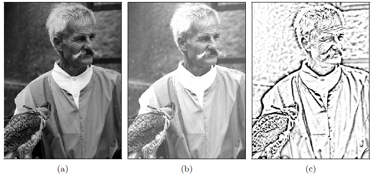

Are the above images "the same"? In the original image (a) and the other five images (b-f), a large distance value will be obtained by simply comparing the difference between image pixels.

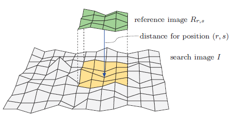
The basic principle of template matching. Taking the origin of the two images as the reference point, the reference image r translates (r,s) units in the image I to be searched, and the size of the image to be searched and the size of the template image determine the maximum search area.
2. Template matching in gray image
Template matching in gray image is mainly to find the same or most similar position of the sub image in template image r and search image I. The following formula represents the offset (r,s) unit of the template in the original image,
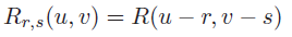
If the reference image r translates R and s units in the horizontal method and vertical direction respectively, the problem of template matching can be summarized as follows:
Given search image I and template image R. Find the reference image after translation and the position with the maximum similarity of the corresponding sub image in the search image.
2.1 distance function in image matching
The most important thing in template matching is to find a similarity measurement function with good robustness to gray and contrast changes.
In order to measure the similarity between images, we calculate the "distance" d(r,s) between the reference image and the corresponding sub image in the search image after each translation (r,s) (as shown in the figure below). The measurement functions in two-dimensional gray-scale images are as follows:
Representation of distance measurement function in two-dimensional image
Sum ofabsolute differences:

Maximumdifference:

Sum ofsquared differences:

Due to the characteristics of SSD function, it is often used in the field of statistics and optimization. In order to find the best matching position of the reference image in the search image, just make the SSD function obtain the minimum value. Namely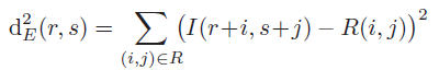

In the above formula, B is the sum of squares of gray values of all pixels in the reference image, which is a constant (independent of r,s), so it can be ignored when calculating its minimum value. A(r,s) represents the sum of squares of gray values of all pixels in the sub image of the search image in (r,s), and C(r,s) is called the linear cross-correlation function of the search image and the reference image, It can usually be expressed as:
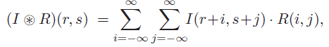
When R and I exceed the boundary, their values are zero, so the above formula can also be expressed as:

If we assume that A(r,s) is a constant in the search image, its value can be ignored when calculating its best matching position in SSD, and when C(r,s) reaches the maximum value, the reference image is most similar to the sub image in the search image. In this case, the minimum value of SSD can be obtained by calculating the maximum value of C(r,s).
2.2 normalized cross correlation
In practical application, the above assumption that A(r,s) is a constant is not always true. Therefore, the above cross-correlation results will change greatly with the change of pixel gray value in the search image. Normalized cross-correlation takes into account the energy of the reference image and the current sub image:
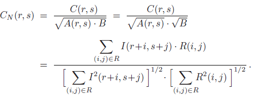
When the gray values of the reference image and the sub image of the search image are positive, the value of Cn(r,s) is always within the range of [0,1], which is independent of the gray values of other pixels of the image. When Cn(r,s) is equal to 1, it indicates that the reference image and sub image reach the maximum similarity at the translation position (r,s); on the contrary, when Cn(r,s) is equal to 0, it indicates that the reference image and sub image do not match at the translation position (r,s). When all gray values in the sub image change, the normalized cross-correlation Cn(r,s) will also change greatly.
2.2 correlation coefficient
In order to solve the above problem, we introduce the gray average value in sub image and template image. The above normalization function can be rewritten as:
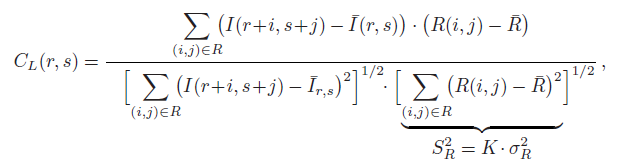
The average values of sub images and reference images are defined as:
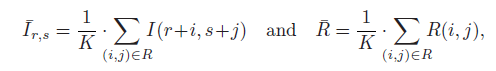
Where K represents the number of pixels in the reference image. In statistics, the above expression is called correlation coefficient. However, different from the global measurement method in statistics, CL(r,s) is defined as a local measurement function. The range of CL(r,s) is [- 1,1]. When CL(r,s) is equal to 1, it indicates that the reference image and sub image reach the maximum similarity at the translation position (r,s); on the contrary, when CL(r,s) is equal to 0, Indicates that at the translation position (r,s), the reference image and sub image do not match at all. Expression:

It represents the variance of pixel gray value in K-times template image R, which is a constant and only needs to be calculated once. The variance has the following relationship: (for details, please refer to http://imagej.net/Integral_Image_Filters)
The details are as follows:

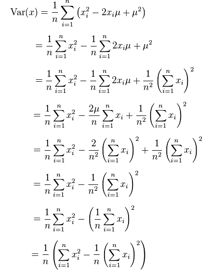
Therefore, SR can be rewritten as

Brought into CL(r,s), you can get:

Thus, an efficient method for calculating the correlation coefficient can be obtained.
2, Source code
% clear
addpath(genpath(pwd)); %Add all files under subfolders
%%Load image
start=6212;
% state=num+1;
% start=6540;
state=1;
% for num = state:294
close all
num = 1 ; %Read the page under the folder num Picture
% 20
%
fname=['Sample library\IMG_',num2str(start+num),'.jpg'];
% There are three license plate folders:'PlateImages/%d.jpg' perhaps'PlateImages/Image1/%d.jpg' or'PlateImages/Image2/%d.jpg'
filename = fullfile(pwd, fname);
Img = imread(filename);
%{
figure(5);
subplot(2,2,1);imshow(Img);title('Original drawing');I1=rgb2gray(Img);
subplot(2,2,2);imshow(I1);title('Grayscale image');
subplot(2,2,3);imhist(I1);title('Gray histogram');I2=edge(I1,'roberts',0.15,'both');
subplot(2,2,4);imshow(I2);title('roberts Operator edge detection')
se=[1;1;1];
I3=imerode(I2,se);
figure(6);
subplot(2,2,1);imshow(I3);title('Image after corrosion');se=strel('rectangle',[25,25]);I4=imclose(I3,se);
subplot(2,2,2);imshow(I4);title('Smooth the outline of the image');I5=bwareaopen(I4,2000);
subplot(2,2,3);imshow(I5);title('Remove small objects from objects');
%}
GetDB;
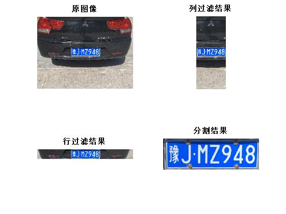
%% Locate license plate
% Locate the license plate: find the location of the license plate in the original picture
% input parameter Img: Read original true color image information
% Output parameters plate: After location processing, from the original true color image(Will be compressed)True color image information at the intercepted license plate position
plate = Pre_Process(Img);
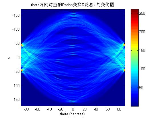
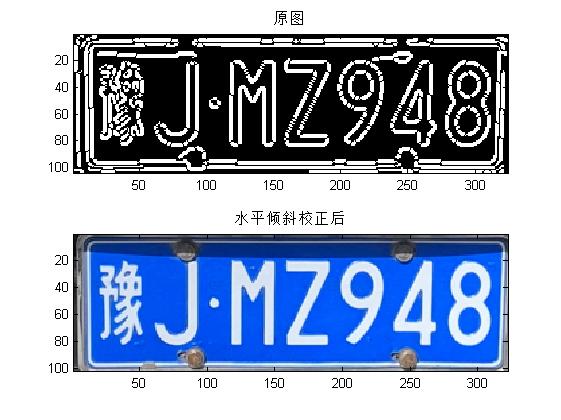
%% Tilt correction
% Tilt correction: the tilt correction of the number to be identified is used separately Radon The transformation and affine function deal with horizontal tilt correction and vertical tilt correction
% Input parameters: plate True color license plate image information intercepted for positioning
% Output parameters:
plate = radon_repair(plate);
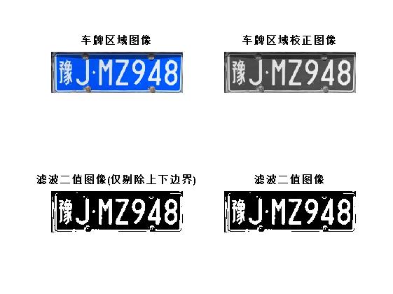
%% License plate filtering
% License plate filtering: culling(Set pixel value to 0)Boundary image information of license plate picture
% Input parameters: plate True color license plate image information intercepted for positioning
% Output parameters: d Filter the original license plate image(That is, excluding the upper and lower boundaries(And using polygon region culling))After the picture, p True color original license plate image plate Picture after counterclockwise rotation
[d, p] = Plate_Process(plate,fname);
%% Split license plate
% Split license plate: cut off(delete)Boundary of license plate image information
% Input parameters: d Filter the original license plate image(That is, excluding the upper and lower boundaries(And using polygon region culling))After the picture, p True color original license plate image plate Picture after counterclockwise rotation
% Output parameters: according to image d Non-0 boundary, cropped input picture: input picture d Output picture after clipping e,Input picture p Output picture after clipping p
[e, p] = Segmation(d, p);
%% Noise removal
function [result, plate] = Plate_Process(plate, fname, flag)
% Split step
if nargin < 3
flag = 1;
end
% n = ndims(A) returns the number of dimensions in the array A.
if ndims(plate) == 3
% I = rgb2gray(RGB) converts the truecolor image RGB to the grayscale intensity image I.
% rgb2gray converts RGB images to grayscale by eliminating the hue and saturation information while retaining the luminance.
plate1 = rgb2gray(plate); % Convert the original picture information of the license plate into grayscale intensity image(Grayscale image? For convenience, the following are called gray images)
else
plate1 = plate;
end
Im = plate1; % Im Is a grayscale image
plate = double(plate);
% B = mean2(A) computes the mean of the values in A.
% b = std2(A) computes the standard deviation of the values in A.
% Find the current picture[Mean standard deviation]Matrix for and database[Mean standard deviation]The matrix is calculated, and then the database parameter information most suitable for processing the current picture is found
m = [mean2(plate(:,:,1)) mean2(plate(:,:,2)) mean2(plate(:,:,3)) std2(plate(:,:,1)) std2(plate(:,:,2)) std2(plate(:,:,3))];
% f = fullfile(filepart1,...,filepartN) builds a full file specification, f, from the folders and file names specified.
% f = fullfile('myfolder','mysubfolder','myfile.m') ===> f = myfolder\mysubfolder\myfile.m
load('model.mat');
ms = cat(1, M.m); % In database[Mean standard deviation]matrix
% B = repmat(A,m,n) creates a large matrix B consisting of an m-by-n tiling of copies of A.
% The size of B is [size(A,1)*m, (size(A,2)*n]. The statement repmat(A,n) creates an n-by-n tiling.
m = repmat(m, size(ms, 1), 1); % The of the current picture[Mean standard deviation]The matrix is expanded to communicate with the database[Mean standard deviation]Matrix operation
% B = sum(A,dim) sums along the dimension of A specified by scalar dim. The dim input is an integer value from 1 to N,
% where N is the number of dimensions in A. Set dim to 1 to compute the sum of each column, 2 to sum rows, etc.
% Sum by row
dis = sum((m - ms).^2, 2); % Current picture[Mean standard deviation]Matrix and database[Mean standard deviation]Variance of matrix
[~, id] = min(dis); % Find the one with the least variance, that is, find the database parameter that is most suitable for processing the current picture
if fname(6)=='s'
ro = M(id).ro; % Angle parameter of picture rotation, in degrees
else
ro=0;
end
th = M(id).th; % The threshold for converting a gray image into a binary image. If the value in the gray image is greater than the threshold, it is converted to 1, otherwise it is converted to 0
pts = M(id).pts; % Defines the vertices of the picture
% B = imrotate(A,angle,method) rotates image A by angle degrees in a counterclockwise direction around its
% center point, using the interpolation method specified by method.
Im = imrotate(Im, ro, 'bilinear'); % Grayscale image Im Rotate counterclockwise ro Degree, the interpolation method is bilinear interpolation
plate = imrotate(plate, ro, 'bilinear'); % Rotate the original image of the license plate counterclockwise ro Degree, the interpolation method is bilinear interpolation
% BW = im2bw(I, level) converts the grayscale image I to a binary image.
% The output image BW replaces all pixels in the input image with luminance(brightness) greater than level with the value 1 (white)
% and replaces all other pixels with the value 0 (black). Specify level in the range [0,1]. This range is relative to
% the signal levels possible for the image's class. Therefore, a level value of 0.5 is midway between black and white, regardless of class.
bw = im2bw(Im, th); % Grayscale image Im Convert to binary image, the conversion threshold is th
% h = fspecial('average', hsize) returns an averaging filter h of size hsize.
% The argument hsize can be a vector specifying the number of rows and columns in h, or it can be a scalar, in which case h is a square matrix.
h = fspecial('average', 2); % Define a multidimensional mean filter h,Dimension is 2 x 2
% B = imfilter(A,h) filters the multidimensional array A with the multidimensional filter h.
% The array A can be logical or a nonsparse numeric array of any class and dimension. The result B has the same size and class as A.
% ___= imfilter(___,options,...) performs multidimensional filtering according to the specified options.
% 'replicate' ===> Input array values outside the bounds of the array are assumed to equal the nearest array border value.
bw1 = imfilter(bw, h, 'replicate'); % Using multidimensional mean filter h,For binary images bw For filtering, the filtering options are replicate
% mask = Mask_Process(bw1); % The function of this method is to remove bw1 The upper and lower miscellaneous lines of the image, that is, use a specific algorithm to eliminate the binary image bw1 Information at the upper and lower boundaries of(The pixel values of these rows are all set to 0)
% Here mask It can be understood that if the image pixel is between the boundary of the clutter line and the upper boundary of the license plate or between the lower boundary of the clutter line and the lower boundary of the license plate, the value of this pixel is 0,
% Otherwise, if the image pixel is between the clutter line boundary and the clutter line lower boundary, the value of this pixel is 1
% bw2 = bw1 .* mask; % this.*Operation can be understood as: and operation, so bw2 Is to use mask Matrix culling binary image bw1 Results after medium interference
bw2 = bw1;
% Except through Mask_Process()In addition to removing miscellaneous lines, if the license plate boundary information is defined, the license plate boundary information can be further used for image processing
% if ~isempty(pts) % If pts Not empty(That is, there is an outer boundary vertex definition),Then execute
% % BW = roipoly(I, c, r) returns the region of interest(ROI) specified by the polygon(polygon) described by vectors c and r,
% % which specify the column and row indices of each vertex(vertex), respectively. c and r must be the same size.
% % According to binary image bw2,And the vertices of the polygon pts(:, 1), pts(:, 2),Get binary image mask,The value of the area surrounded by vertices is all 1,
% % The values of other areas are all 0. The purpose of this is to eliminate the interference of license plate boundary
% mask = roipoly(bw2, pts(:, 1), pts(:, 2)); % Get one by pts vertex(Composable polygon)Specified binary boundary image
% bw1 = bw1 .* mask; % bw1 It is a binary image that only uses polygons to eliminate interference
% bw2 = bw2 .* mask; % bw2 Is to use Mask_Process()Algorithm and polygon are two methods to eliminate the interference of binary image
% end3, Operation results