6.3 image coding technology and standard of Python image processing - wavelet transform coding

1 algorithm principle

The so-called wavelet is small for Fourier waves, Fourier wave refers to sine wave (or cosine wave) that oscillates infinitely in time domain. Relatively speaking, wavelet refers to a wave with very concentrated energy in time domain. Its energy is limited, concentrated near a certain point, and the integral value is zero, which shows that it is an orthogonal wave like Fourier wave. The steps of wavelet transform are as follows:

1) compare the wavelet w(t) with the beginning of the original function f(t) and calculate the coefficient C. Coefficient C represents the similarity between this part of the function and wavelet;

2) shift the wavelet to the right by K units to obtain the wavelet w(t-k), repeat 1. Repeat this step until function f ends;

3) extend wavelet w(t) to obtain wavelet w(t/2), and repeat steps 1 and 2;

Continuously expand the wavelet and repeat 1,2,3.

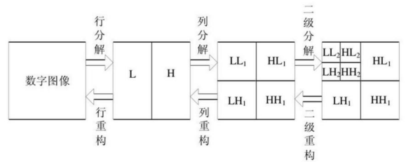
The two-dimensional discrete wavelet decomposition and reconstruction process of the image is shown in the figure below,

The decomposition process can be described as follows: first, 1D-DWT is performed on each row of the image to obtain the low-frequency component L and high-frequency component H in the horizontal direction of the original image, and then 1D-DWT is performed on each column of the transformed data to obtain the low-frequency component LL in the horizontal and vertical directions, the low-frequency component LH in the horizontal direction and the high-frequency component H in the vertical direction of the original image High frequency in the horizontal direction and low frequency HL in the vertical direction and high frequency component HH in the horizontal and vertical directions.

The reconstruction process can be described as follows: first, inverse discrete wavelet transform is performed on each column of the transformation result, and then one-dimensional inverse discrete wavelet transform is performed on each row of the transformed data to obtain the reconstructed image. It can be seen from the above process that the wavelet decomposition of the image is a process of separating the signal according to low frequency and directed high frequency. In the decomposition process, the LL component can be further decomposed according to the needs until the requirements are met.

2 code

Run code description

1. Change the picture address in the code (the address cannot have Chinese)

Change the path put(r'../image/image1.jpg') in the put(path) function

2. Pay attention to the last plt Savefig ('1. New. JPG ') is to save the plt image. If it is not used, it can be commented out

Code dependent packages:

matplotlib  3.4.2
numpy  1.20.3
opencv-python  4.1.2.30
PyWavelets  1.1.1

# pip installation
pip install matplotlib numpy opencv-python PyWavelets

import cv2
import numpy as np
import matplotlib.pyplot as plt
# python wavelet analysis library PyWavelets needs to be installed
from pywt import dwt2, idwt2

def put(path):
    # 0 indicates that the grayscale image is read directly
    img = cv2.imread(path, 0)
    
    # haar wavelet transform for img:, haar wavelet
    cA, (cH, cV, cD) = dwt2(img, 'haar')

    # After wavelet transform, the image corresponding to the low-frequency component:
    a = np.uint8(cA / np.max(cA) * 255)
    # After wavelet transform, the image corresponding to the high-frequency component in the horizontal direction:
    b = np.uint8(cH / np.max(cH) * 255)
    # After wavelet transform, the image corresponding to the vertical square high-frequency component:
    c = np.uint8(cV / np.max(cV) * 255)
    # After wavelet transform, the image corresponding to the diagonal high-frequency component:
    d = np.uint8(cD / np.max(cD) * 255)

    # Reconstructed image according to wavelet coefficients
    rimg = idwt2((cA, (cH, cV, cD)), 'haar')

    plt.rcParams['font.sans-serif'] = ['SimHei']
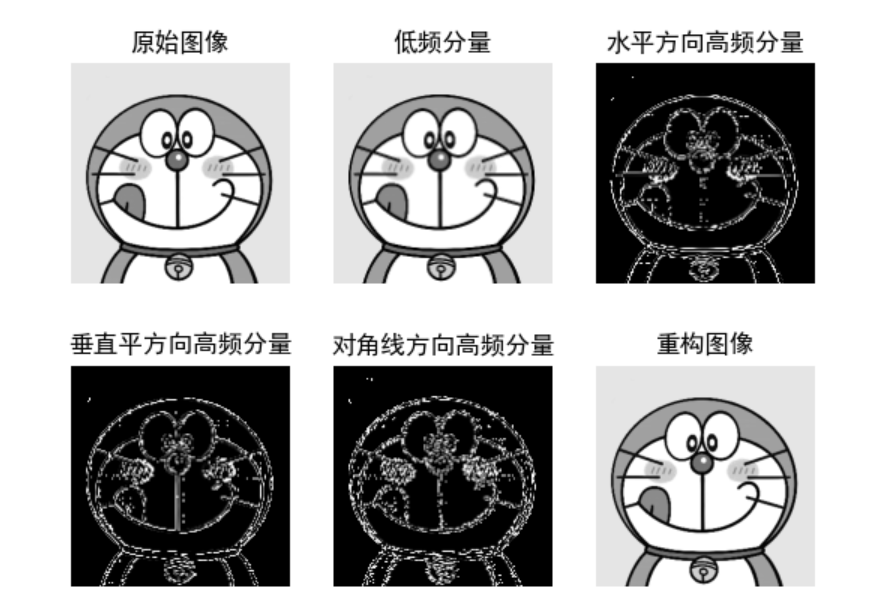
    plt.subplot(231), plt.imshow(img, 'gray'), plt.title('original image '), plt.axis('off')
    plt.subplot(232), plt.imshow(a, 'gray'), plt.title('Low frequency component'), plt.axis('off')
    plt.subplot(233), plt.imshow(b, 'gray'), plt.title('Horizontal high frequency component'), plt.axis('off')
    plt.subplot(234), plt.imshow(c, 'gray'), plt.title('Vertical square high frequency component'), plt.axis('off')
    plt.subplot(235), plt.imshow(d, 'gray'), plt.title('Diagonal high frequency component'), plt.axis('off')
    plt.subplot(236), plt.imshow(rimg, 'gray'), plt.title('Reconstructed image'), plt.axis('off')

    # plt.savefig('3.new-img.jpg')
    plt.show()


# Image processing function, path to be passed in
put(r'../image/image1.jpg')

3 Effect