In the first issue, we explained and realized the most basic linear regression. In this issue, we will talk about the regression problem to the classification problem. At this time, we need to add some elements based on the linear regression model, that is activation function so that our model can solve nonlinear data and classification problems.
Previous highlights:
Hand to hand neural network explanation and no packet switching implementation series (1) linear regression [R language] [Xiaobai learning notes]
I. model explanation
1. Hypothesis Function
Suppose there are n data points, 4 features and 3 categorical variables in a set of data. Our purpose is to learn the features of existing data by establishing a mathematical model and finally accurately predict the target variables. Because the categorical variables are different and special from continuous variables, we need to encode the categorical variables one hot before training the model Let's take a simple example. For example, our target classification variable is to distinguish fruit [Apple] 🍎, Banana 🍌, orange 🍊], The one hot encoded variable will become like this
[🍎: (1,0,0), 🍌: (0,1,0),🍊: (0,0,1)].
After completing the above coding, we will start to explain the theory of Softmax regression model. According to the framework of neural network, Softmax regression is actually a neural network with only one layer of fully connected/dense layer.
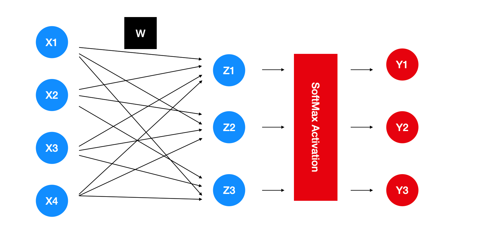 The data cases mentioned above will be directly brought into the model as shown in the chart. The chart does not draw the deviation, but we default to the existence of the deviation. The steps represented by red will be described in the activation function section.
If you write the blue steps in the chart into a mathematical formula,
z
1
=
x
1
w
11
+
x
2
w
12
+
x
3
w
13
+
x
4
w
14
+
b
1
,
z
2
=
x
1
w
21
+
x
2
w
22
+
x
3
w
23
+
x
4
w
24
+
b
2
,
z
3
=
x
1
w
31
+
x
2
w
32
+
x
3
w
33
+
x
4
w
34
+
b
3
,
z_1 = x_1w_{11} + x_2w_{12} + x_3w_{13} + x_4w_{14} + b_1, \\ z_2 = x_1w_{21} + x_2w_{22} + x_3w_{23} + x_4w_{24} + b_2, \\ z_3 = x_1w_{31} + x_2w_{32} + x_3w_{33} + x_4w_{34} + b_3,
z1=x1w11+x2w12+x3w13+x4w14+b1,z2=x1w21+x2w22+x3w23+x4w24+b2,z3=x1w31+x2w32+x3w33+x4w34+b3,
among
w
w
w is the weight parameter [weights] of the model,
b
b
b is the deviation [bias/intercept].
In order to make the calculation more concise, the formula is vectorized,
Z
=
X
W
+
b
,
Z = XW + b,
Z=XW+b,
here
Z
Z
Z is our hypothetical function.
It also hides the deviation value in the
w
w
w is further simplified,
Z
=
X
W
,
\boxed{Z = XW} ,
Z=XW,
According to the above data case,
Z
=
[
1
0
0
0
1
0
.
.
.
.
.
.
.
.
.
0
0
1
]
,
X
=
[
1
x
11
x
12
x
13
x
14
.
.
.
.
.
.
.
.
.
.
.
.
.
.
.
1
x
n
1
x
n
2
x
n
3
x
n
4
]
,
W
=
[
b
1
b
2
b
3
w
11
w
21
w
31
w
12
w
22
w
32
w
13
w
23
w
33
w
14
w
24
w
34
]
Z = \begin{bmatrix} 1 & 0 & 0 \\ 0 & 1 & 0 \\ ... & ... & ... \\ 0 & 0 & 1 \end{bmatrix}, X = \begin{bmatrix} 1 & x_{11} & x_{12} &x_{13} &x_{14}\\ ... & ... & ... & ... & ... \\ 1 & x_{n1} & x_{n2} & x_{n3} &x_{n4} \end{bmatrix}, W = \begin{bmatrix} b_1 & b_2 & b_3 \\ w_{11} & w_{21} & w_{31} \\ w_{12} & w_{22} & w_{32} \\ w_{13} & w_{23} & w_{33} \\ w_{14} & w_{24} & w_{34} \end{bmatrix}
Z=⎣⎢⎢⎡10...001...000...1⎦⎥⎥⎤,X=⎣⎡1...1x11...xn1x12...xn2x13...xn3x14...xn4⎦⎤,W=⎣⎢⎢⎢⎢⎡b1w11w12w13w14b2w21w22w23w24b3w31w32w33w34⎦⎥⎥⎥⎥⎤.
If our data has n data points, m features and K classification variables, then
X
X
X will be a
n
∗
(
m
+
1
)
n*(m+1)
Matrix of n * (m+1),
W
W
W will be a
(
m
+
1
)
∗
K
(m+1)*K
Matrix of (m+1) * K, last
Z
Z
Z will be a
n
∗
K
n*K
Matrix of n * K.
2 Activation Function
If we use linear regression, the above hypothetical function is sufficient. But what we want to solve this time is the classification problem, so we need some additional steps to change the linear formula to calculate a new quantitative value to predict the classification variables, and the probability will naturally become the most appropriate quantitative value! So the first step is to calculate Z Z After Z, a new function will be needed to convert it into probability. This step is usually called activation (the red part in the figure above). The activation function used this time is Softmax function, which was first used by a social scientist named R. Duncan Luce in 1959. The name of our model comes from this. The function formula is as follows,
y
^
j
=
e
x
p
(
Z
j
)
∑
j
=
1
K
e
x
p
(
Z
j
)
,
\boxed{\hat{y}_j = \frac{exp(Z_j)}{\sum_{j=1}^{K} exp(Z_j)} },
y^j=∑j=1Kexp(Zj)exp(Zj),
among
y
^
j
\hat{y}_j
y ^ j is the calculated prediction probability,
K
K
K represents the number of target classification variables,
j
j
j is the index of the target classification variable. The denominator is to ensure that the conversion probability can only have a range of 0-1.
3 Loss Function
When training the model, we will need the loss function to quantify the prediction error. At the same time, the loss function used in the classification problem will be different from that used in the regression problem. When calculating the probability of the following true classification,
P
(
Y
^
∣
X
)
=
∏
i
=
1
n
P
(
y
^
(
i
)
∣
x
(
i
)
)
.
P(\hat{Y}|X) = \prod_{i=1}^{n} P(\hat{y}^{(i)}|x^{(i)}).
P(Y^∣X)=i=1∏nP(y^(i)∣x(i)).
According to the logic of maximum likelihood estimation, our goal is to P ( Y ^ ∣ X ) P(\hat{Y}|X) P(Y ^∣ X) maximizes, but due to P ( Y ^ ∣ X ) P(\hat{Y}|X) P(Y ^ ∣ X) is composed of a series of products. It will become extremely difficult to find the derivative. At this time, through l o g log Log (here) l o g log log is the natural logarithm l n ln ln) property, we can convert the product into a sum, and because l o g log Log is a monotonic increasing function, so the answer obtained from log likelihood will answer the original likelihood value at the same time. Finally, because the habit of machine learning is to minimize the problem, when we want to maximize it P ( Y ^ ∣ X ) P(\hat{Y}|X) When P(Y ^∣ X), it is relatively − l o g P ( Y ^ ∣ X ) -logP(\hat{Y}|X) − logP(Y ^∣ X) minimized,
−
l
o
g
P
(
Y
^
∣
X
)
=
∑
i
=
1
n
−
l
o
g
P
(
y
^
(
i
)
∣
x
(
i
)
)
=
∑
i
=
1
n
l
(
y
^
(
i
)
,
y
(
i
)
)
,
-logP(\hat{Y}|X) = \sum_{i=1}^{n}-logP(\hat{y}^{(i)}|x^{(i)}) = \sum_{i=1}^{n} l(\hat{y}^{(i)}, y^{(i)}),
−logP(Y^∣X)=i=1∑n−logP(y^(i)∣x(i))=i=1∑nl(y^(i),y(i)),
Here we finally determine our loss function
l
(
y
^
(
i
)
,
y
(
i
)
)
l(\hat{y}^{(i)}, y^{(i)})
l(y^(i),y(i)),
l
(
y
^
(
i
)
,
y
(
i
)
)
=
−
∑
j
=
1
K
y
j
l
o
g
y
^
j
.
\boxed{l(\hat{y}^{(i)}, y^{(i)}) = -\sum_{j=1}^{K} y_j log\hat{y}_j}.
l(y^(i),y(i))=−j=1∑Kyjlogy^j.
There are several points that deserve special attention. First, the loss function above is famous in Shannon's information theory Cross entropy [cross entry]. The second point is
y
j
y_j
yj , is our real classification target. At the beginning, we used one hot coding for classification variables (e.g[ 🍎: (1,0,0), 🍌: (0,1,0), 🍊: (0, 0, 1)], so when calculating
y
j
l
o
g
y
^
j
y_j log\hat{y}_j
When yj log ^ j, only the correct classification prediction probability can be saved, and other incorrect classifications will be equal to
0
0
0.
4 derivation of stochastic gradient descent method
This time, we will also use the small batch random gradient descent method to find the model parameters of the optimal solution
W
W
W. Therefore, we need to solve the partial derivative
∂
l
∂
W
\frac{\partial l}{\partial W}
∂W∂l. Note, however, that the loss function
l
l
l is a composite function, from
y
^
\hat{y}
y ^ to
Z
Z
Z to
W
W
W is set down step by step and written into a mathematical equation
l
(
y
^
(
i
)
,
y
(
i
)
)
=
l
(
SoftMax
(
Z
(
W
)
)
,
y
(
i
)
)
l(\hat{y}^{(i)}, y^{(i)}) = l(\text{SoftMax}(Z(W)), y^{(i)})
l(y ^ (i),y(i))=l(SoftMax(Z(W)),y(i)), then the chain rule becomes very convenient,
∂
l
∂
W
=
∂
l
∂
Z
∂
Z
∂
W
.
\frac{\partial l}{\partial W} = \frac{\partial l}{\partial Z} \frac{\partial Z}{\partial W}.
∂W∂l=∂Z∂l∂W∂Z.
Before deriving, the loss function is transformed into
Z
Z
Function of Z,
l
(
y
^
(
i
)
,
y
(
i
)
)
=
−
∑
j
=
1
K
y
j
l
o
g
e
x
p
(
Z
j
)
∑
k
=
1
K
e
x
p
(
Z
k
)
,
l
(
y
^
(
i
)
,
y
(
i
)
)
=
−
∑
j
=
1
K
y
j
Z
j
+
∑
j
=
1
K
y
j
l
o
g
(
∑
k
=
1
K
e
x
p
(
Z
k
)
)
,
l(\hat{y}^{(i)}, y^{(i)}) = -\sum_{j=1}^{K} y_j log \frac{exp(Z_j)}{\sum_{k=1}^{K} exp(Z_k)}, \\ l(\hat{y}^{(i)}, y^{(i)}) = -\sum_{j=1}^{K} y_j Z_j + \sum_{j=1}^{K} y_j log(\sum_{k=1}^{K} exp(Z_k)),
l(y^(i),y(i))=−j=1∑Kyjlog∑k=1Kexp(Zk)exp(Zj),l(y^(i),y(i))=−j=1∑KyjZj+j=1∑Kyjlog(k=1∑Kexp(Zk)),
In the second step, we use the log feature again to simplify the formula, and then there are two indexes
j
j
j and
k
k
k. They are all calculating the sum of classified variables, but they need to be distinguished before using different indexes. what's more
∑
j
=
1
K
y
j
\sum_{j=1}^{K} y_j
∑ j=1K and ∑ yj = 1 (because of one hot coding),
l
l
The final formula of l is as follows,
l
=
l
o
g
(
∑
k
=
1
K
e
x
p
(
Z
k
)
)
−
∑
j
=
1
K
y
j
Z
j
.
l = log(\sum_{k=1}^{K} exp(Z_k)) - \sum_{j=1}^{K} y_j Z_j .
l=log(k=1∑Kexp(Zk))−j=1∑KyjZj.
The rest is derivation,
∂
l
∂
Z
=
1
∑
k
=
1
K
e
x
p
(
Z
k
)
e
x
p
(
Z
k
)
−
y
j
=
Softmax
(
Z
j
)
−
y
j
=
y
^
j
−
y
j
,
∂
Z
∂
W
=
∂
∂
W
(
X
(
i
)
W
)
=
X
(
i
)
,
∂
l
∂
W
=
∂
l
∂
Z
∂
Z
∂
W
=
X
(
i
)
(
y
^
j
−
y
j
)
.
\frac{\partial l}{\partial Z} = \frac{1}{\sum_{k=1}^{K} exp(Z_k)} exp(Z_k) - y_j = \text{Softmax}(Z_j) - y_j = \hat{y}_j - y_j,\\ \frac{\partial Z}{\partial W} = \frac{\partial }{\partial W} (X^{(i)}W) = X^{(i)},\\ \boxed{\frac{\partial l}{\partial W} = \frac{\partial l}{\partial Z} \frac{\partial Z}{\partial W} = X^{(i)}(\hat{y}_j - y_j)} .
∂Z∂l=∑k=1Kexp(Zk)1exp(Zk)−yj=Softmax(Zj)−yj=y^j−yj,∂W∂Z=∂W∂(X(i)W)=X(i),∂W∂l=∂Z∂l∂W∂Z=X(i)(y^j−yj).
As like as two peas, the students who are eyes and eyes will find that the partial derivative is exactly the same as that of the linear regression model. Yes, the partial derivative of all exponential family distribution models will be this result, and the only change is
y
^
\hat{y}
y^.
Next, the parameters of the model are updated according to the random gradient descent method
W
W
W,
W
=
W
−
η
β
∑
i
∈
β
∇
W
l
(
i
)
(
W
)
,
W
=
W
−
η
β
∑
i
∈
β
X
(
i
)
(
y
^
j
−
y
j
)
,
W = W - \frac{\eta}{\beta}\sum_{i \in \beta} \nabla_{W} l^{(i)}(W) ,\\ \boxed{W = W - \frac{\eta}{\beta}\sum_{i \in \beta} X^{(i)}(\hat{y}_j - y_j) },
W=W−βηi∈β∑∇Wl(i)(W),W=W−βηi∈β∑X(i)(y^j−yj),
here
η
\eta
η Is the learning rate,
β
\beta
β batch size.
5 algorithm summary
The steps to be realized are summarized as follows,
- Randomly generate weight parameters ( W , b ) (W,b) (W,b).
- Calculation assumption function Z = X W Z = XW Z=XW.
- activation Z Z Z is calculated y ^ = e x p ( Z j ) ∑ j = 1 K e x p ( Z j ) \hat{y} = \frac{exp(Z_j)}{\sum_{j=1}^{K} exp(Z_j)} y^=∑j=1Kexp(Zj)exp(Zj).
- One - step batch random gradient descent method
- to update ( W , b ) (W,b) (W,b), W = W − η β ∑ i ∈ β X ( i ) ( y ^ j − y j ) W = W - \frac{\eta}{\beta}\sum_{i \in \beta} X^{(i)}(\hat{y}_j - y_j) W=W−βη∑i∈βX(i)(y^j−yj)
- Repeat 2-5 until the preset cycle or other preset conditions are reached.
II. Data
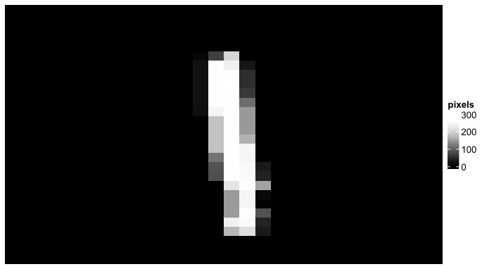
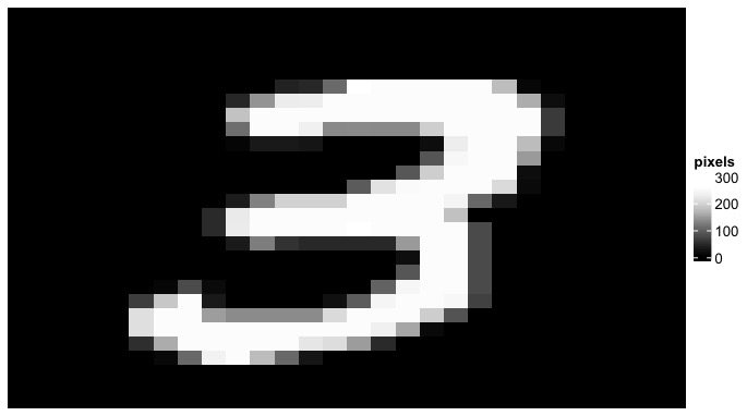
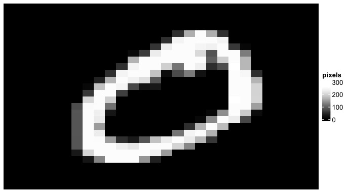
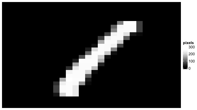
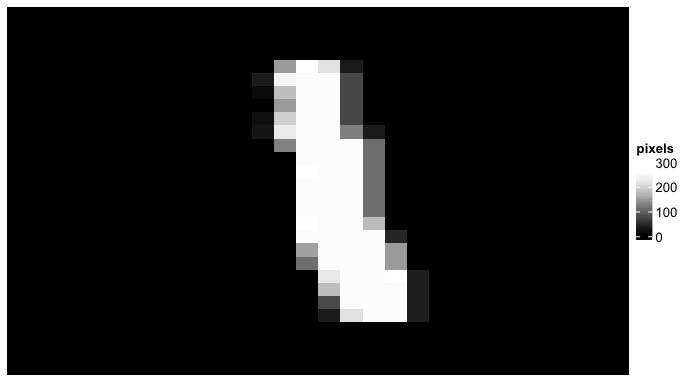
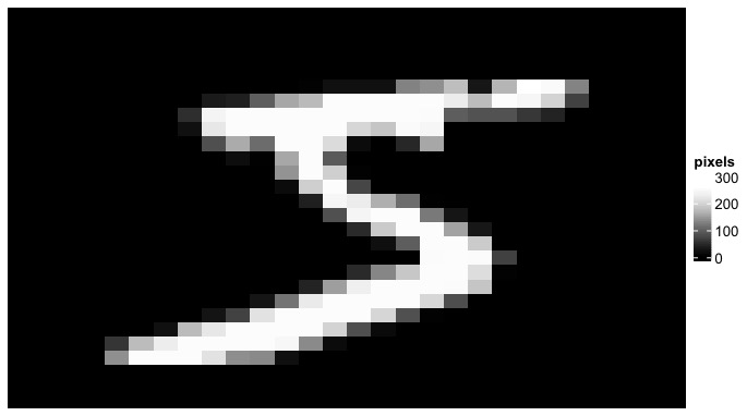
After explaining the principle of the model, we will first understand the data used this time, This is the famous MNIST database of handwritten numeral (0-9) classification. Each data point is a 28x28 black-and-white picture. Our goal is to use Softmax return to realize simple computer vision [computer vision] model, that is, let AI determine which number from 0 to 9 is written in the picture. The first step will be to download MNIST database and data visualization from Keras package.
library(tidyverse)
library(matrixStats)
library(tensorflow)
library(keras)

library(RColorBrewer)
# install.packages('ComplexHeatmap')
library(ComplexHeatmap)


# ---------------------------- Load the Data -------------------------------
# Digit dataset
mnist = dataset_mnist()
X_train = mnist$train$x
Y_train = mnist$train$y
X_test = mnist$test$x
Y_test = mnist$test$y

# VIZ the image:
PlotImage = function(image_array) {
  digit_color = colorRampPalette(rev(brewer.pal(n=9,
                                                name = "Greys")))(100)
  Heatmap(image_array, name= 'pixels',
          col = digit_color,
          cluster_rows = F, cluster_columns = F,
          border = F, column_names_rot = 90
  )
}

for (i in 1:10) {
  image = X_train[i, , ]
  print(PlotImage(image))
}
– code output:


Before training the model with the original data, the original data needs further processing. The first step is to flatten all 28x28 picture data into a nxm matrix, where n represents the number of pictures and m represents the number of pictures
28
∗
28
=
784
28*28 = 784
28 * 28 = 784 pixel features. After flattening the data, the next step is to divide the data by the highest pixel value (255) to standardize it into a range of 0-1. The remaining note is to add a column vector of all 1 before the first column of the flattened matrix to make the deviation value
b
b
b integration
W
W
W inside. Finally, the digital target of the picture is one-hot encoded (using the 'to_category' function in Keras).
# ---------------------------- Data Processing -------------------------------
## Flatten the 2D image into 1D features:
X_train_mat = matrix(0,  nrow = nrow(X_train), ncol = 28*28 )
for (i in 1:nrow(X_train)){
  # also normalize the pixel value by dividing 255
  X_train_mat[i, ] = matrix(X_train[i, , ], ncol = 28*28, byrow = TRUE) / 255
}

X_test_mat = matrix(0, nrow = nrow(X_test), ncol = 28*28 )
for (i in 1:nrow(X_test)){
  # also normalize the pixel value by dividing 255
  X_test_mat[i, ] = matrix(X_test[i, , ], ncol = 28*28, byrow = TRUE) / 255
}

## Add dummy col of value 1 to X for embedding the bias term:
X_train_mat = cbind(rep(1, nrow(X_train_mat)), X_train_mat)
X_test_mat = cbind(rep(1, nrow(X_test_mat)), X_test_mat)

## One-hot encoding for the Label:
Y_train_oh = to_categorical(Y_train)
Y_test_oh = to_categorical(Y_test)

# check training data dimension
dim(X_train_mat)
dim(Y_train_oh)
III. model implementation
After completing the data transformation, let's start to implement the Softmax regression model. Start with simple hypothetical functions and Softmax activation functions.
Hypothesis = function(X, w) {
  ## Hypothesis function: Z = XW + b
  # Notice: b is already embedded within W as the first column
  return(X %*% w )
}

Softmax = function(Z){
  ## Softmax activation: exp(Z) / Row Summation (exp(Z))
  return( exp(Z) / rowSums(exp(Z)) )
}
Next, write the cross entropy of the loss function. At the same time, we will add an assistant function that can calculate the prediction accuracy. Note that the cross entropy needs the target value after one hot coding Y o h Y_{oh} Yoh# and the function of prediction accuracy requires the original target value before one hot coding Y Y Y!
CrossEntropy = function(Y_hat, Y_oh){
  ## Loss function: l(yhat, y) = -summation(yj log yhatj)
  # NOTEL Groud Truth Y need to be one-hot encoded.
  # using the Ground Truth target as index to only select the nonzero class
  # [using normal element wise multiplication instead of matrix multiplication]
  return(-rowSums(log(Y_hat) * Y_oh))
}

ComputeAccuracy = function(Y_hat, Y){
  ## Compute the Accuracy
  # need to subtract 1 here because the target starts with 0!
  pred = apply(Y_hat, MARGIN = 1, FUN = function(x) which.max(x) - 1)
  acc = sum(pred == Y) / length(Y)
  return(acc)
}
The rest is to write the R function of the random gradient descent method. As usual, when running matrix multiplication, be sure to pay attention to the size of the multiplication matrix, otherwise there will be a direct bug. such as X b a t c h X_{batch} Xbatch # is a β ∗ ( m + 1 ) \beta * (m+1) β * matrix sum of (m+1) Y ^ b a t c h − Y b a t c h \hat{Y}_{batch} - Y_{batch} The result of Y^batch − Ybatch is a β ∗ K \beta * K β * the ultimate goal of K matrix is to update W W W and W W W is a ( m + 1 ) ∗ K (m+1)*K (m+1) * K matrix. So one of the methods is transpose X b a t c h X_{batch} Xbatch} assembly ( m + 1 ) ∗ β (m+1)*\beta (m+1)∗ β So that we can sum Y ^ b a t c h − Y b a t c h \hat{Y}_{batch} - Y_{batch} The results of Y^batch − Ybatch are multiplied without error.
SGD = function(X, Y_oh, w, lr, batch_size){
  ## minibatch stochastic gradient descent

  # Minibatch sampling:
  batch_ind = sample(nrow(X), batch_size, replace = FALSE)
  X_batch = X[batch_ind, ]
  Y_batch = Y_oh[batch_ind, ]

  # Compute gradient for the batch sample:
  Z_batch = Hypothesis(X_batch, w)
  Y_hat_batch = Softmax(Z_batch)
  # transpose X for correct dimension
  w_grad = t(X_batch) %*% (Y_hat_batch - Y_batch)

  # Update w
  w = w - lr/batch_size * w_grad

  return(w)

}
After coding all the required functions, we can randomly generate the parameters required by the model, and then start training the model.
# ------------------------- Initiate Models Parameters ---------------------------
n = nrow(X_train_mat) # num of training data points
m = ncol(X_train_mat) # num of features
k = ncol(Y_train_oh) # num of target classes

# Dim(w) = num of features * num of Target Classes
# note: b is also embedded within W as the first column
w = matrix(rnorm(m*k, mean = 0, sd = 0.01),
           nrow = m, ncol = k, byrow = TRUE )
#
batch_size = 512
lr = 0.5
num_epoch = 50
#
net = Hypothesis
active = Softmax
loss = CrossEntropy
#
w_list = list()
l_list = list()
acc_list = list()
# ------------------------------ Train the models --------------------------------
for (epoch in 1:num_epoch ){
  # Update parameters w:
  w = SGD(X_train_mat, Y_train_oh, w, lr, batch_size)
  Y_hat = active(net(X_train_mat, w))
  l = loss(Y_hat, Y_train_oh)
  acc_train = ComputeAccuracy(Y_hat, Y_train)

  # Compute test data accuracy:
  Y_hat_test = active(net(X_test_mat, w))
  acc_test = ComputeAccuracy(Y_hat_test, Y_test)
  ## Accumulate parameters, loss, and accuracy:
  w_list[[epoch]] = w
  l_list[[epoch]] = l
  acc_list[[epoch]] = acc_test

  print(str_c('epoch ', epoch, ' Loss: ', mean(l),
              ' Train Accuracy: ', acc_train, ' Test Accuracy: ', acc_test ))

}
– code output:
[1] "epoch 1 Loss: 2.01185957862662 Train Accuracy: 0.3933 Test Accuracy: 0.3932"
[1] "epoch 2 Loss: 1.79866336994313 Train Accuracy: 0.5837 Test Accuracy: 0.5815"
[1] "epoch 3 Loss: 1.60035098466163 Train Accuracy: 0.692483333333333 Test Accuracy: 0.6981"
[1] "epoch 4 Loss: 1.45199775782509 Train Accuracy: 0.753166666666667 Test Accuracy: 0.7591"
[1] "epoch 5 Loss: 1.32667656580226 Train Accuracy: 0.805016666666667 Test Accuracy: 0.81"
[1] "epoch 6 Loss: 1.23351659868024 Train Accuracy: 0.77195 Test Accuracy: 0.7797"
[1] "epoch 7 Loss: 1.15247059426567 Train Accuracy: 0.790816666666667 Test Accuracy: 0.7965"
[1] "epoch 8 Loss: 1.08940996066825 Train Accuracy: 0.822066666666667 Test Accuracy: 0.832"
[1] "epoch 9 Loss: 1.03435513731771 Train Accuracy: 0.79235 Test Accuracy: 0.7997"
[1] "epoch 10 Loss: 0.992790215169106 Train Accuracy: 0.795583333333333 Test Accuracy: 0.8038"
[1] "epoch 11 Loss: 0.946572561174173 Train Accuracy: 0.824333333333333 Test Accuracy: 0.8357"
[1] "epoch 12 Loss: 0.909750711598293 Train Accuracy: 0.824633333333333 Test Accuracy: 0.831"
[1] "epoch 13 Loss: 0.87881802974624 Train Accuracy: 0.821616666666667 Test Accuracy: 0.8289"
[1] "epoch 14 Loss: 0.856014529247105 Train Accuracy: 0.8227 Test Accuracy: 0.8285"
[1] "epoch 15 Loss: 0.826283243741158 Train Accuracy: 0.8323 Test Accuracy: 0.8393"
[1] "epoch 16 Loss: 0.806752614095863 Train Accuracy: 0.825666666666667 Test Accuracy: 0.8334"
[1] "epoch 17 Loss: 0.783079841221734 Train Accuracy: 0.837433333333333 Test Accuracy: 0.8464"
[1] "epoch 18 Loss: 0.768047193553696 Train Accuracy: 0.841716666666667 Test Accuracy: 0.8497"
[1] "epoch 19 Loss: 0.750615882974677 Train Accuracy: 0.8366 Test Accuracy: 0.8455"
[1] "epoch 20 Loss: 0.735299170805383 Train Accuracy: 0.8377 Test Accuracy: 0.8473"
[1] "epoch 21 Loss: 0.73117605924406 Train Accuracy: 0.84355 Test Accuracy: 0.8519"
[1] "epoch 22 Loss: 0.708800130686964 Train Accuracy: 0.84555 Test Accuracy: 0.8553"
[1] "epoch 23 Loss: 0.696495446607604 Train Accuracy: 0.8493 Test Accuracy: 0.8581"
[1] "epoch 24 Loss: 0.687002815757669 Train Accuracy: 0.840733333333333 Test Accuracy: 0.8477"
[1] "epoch 25 Loss: 0.672860505884358 Train Accuracy: 0.851316666666667 Test Accuracy: 0.8583"
[1] "epoch 26 Loss: 0.664951719016957 Train Accuracy: 0.84635 Test Accuracy: 0.8543"
[1] "epoch 27 Loss: 0.655106062900735 Train Accuracy: 0.849583333333333 Test Accuracy: 0.857"
[1] "epoch 28 Loss: 0.645319103773532 Train Accuracy: 0.852516666666667 Test Accuracy: 0.8607"
[1] "epoch 29 Loss: 0.637838867466701 Train Accuracy: 0.8526 Test Accuracy: 0.8603"
[1] "epoch 30 Loss: 0.631416726867725 Train Accuracy: 0.85445 Test Accuracy: 0.862"
[1] "epoch 31 Loss: 0.624603858639298 Train Accuracy: 0.852833333333333 Test Accuracy: 0.8622"
[1] "epoch 32 Loss: 0.616821827127777 Train Accuracy: 0.85445 Test Accuracy: 0.865"
[1] "epoch 33 Loss: 0.610096882199635 Train Accuracy: 0.857083333333333 Test Accuracy: 0.8655"
[1] "epoch 34 Loss: 0.602093020051617 Train Accuracy: 0.86005 Test Accuracy: 0.8684"
[1] "epoch 35 Loss: 0.596405980525509 Train Accuracy: 0.85895 Test Accuracy: 0.8687"
[1] "epoch 36 Loss: 0.592009076665646 Train Accuracy: 0.861783333333333 Test Accuracy: 0.869"
[1] "epoch 37 Loss: 0.585498505571898 Train Accuracy: 0.861616666666667 Test Accuracy: 0.8695"
[1] "epoch 38 Loss: 0.580217579430339 Train Accuracy: 0.860866666666667 Test Accuracy: 0.8697"
[1] "epoch 39 Loss: 0.575570930764546 Train Accuracy: 0.8636 Test Accuracy: 0.872"
[1] "epoch 40 Loss: 0.570743035290116 Train Accuracy: 0.864333333333333 Test Accuracy: 0.8731"
[1] "epoch 41 Loss: 0.566742974680231 Train Accuracy: 0.861916666666667 Test Accuracy: 0.872"
[1] "epoch 42 Loss: 0.562568722389329 Train Accuracy: 0.862466666666667 Test Accuracy: 0.8722"
[1] "epoch 43 Loss: 0.559576088097929 Train Accuracy: 0.863816666666667 Test Accuracy: 0.8728"
[1] "epoch 44 Loss: 0.555851224868723 Train Accuracy: 0.865266666666667 Test Accuracy: 0.8763"
[1] "epoch 45 Loss: 0.551350385459388 Train Accuracy: 0.86635 Test Accuracy: 0.8767"
[1] "epoch 46 Loss: 0.546167196346621 Train Accuracy: 0.8663 Test Accuracy: 0.8745"
[1] "epoch 47 Loss: 0.542812103779878 Train Accuracy: 0.8683 Test Accuracy: 0.8766"
[1] "epoch 48 Loss: 0.539687741215432 Train Accuracy: 0.869716666666667 Test Accuracy: 0.878"
[1] "epoch 49 Loss: 0.535411556744273 Train Accuracy: 0.869683333333333 Test Accuracy: 0.8791"
[1] "epoch 50 Loss: 0.533269989328817 Train Accuracy: 0.87 Test Accuracy: 0.8778"
For Minist data, modern neural network models can be easily achieved 95 % 95\% About 95% accuracy. From the above results, we can see that our Softmax regression model has reached the goal before and after 50 weeks of training 88 % 88\% The accuracy of about 88% is not as high as expected. If you lengthen the cycle, you can really improve the accuracy to 92 % 92\% About 92% (200 cycles have been tried privately), but the relative model training time will be longer. Another possibility is that our model is too simplistic and does not take into account some factors, such as numerical stability.
Finally, we try the Keras model framework in Tensorflow, one of the most advanced packages, to build the same Softmax regression model, using the same data and the same cycle. The result is 90 % 90\% About 90%, which is really better than our model!
# ------------------------- Test the data on Keras ---------------------------
nn = keras_model_sequential()
nn %>%
  layer_dense(units = 10, input_shape = ncol(X_train_mat),
              activation = 'softmax')

nn %>% compile(
  loss = 'categorical_crossentropy',
  optimizer = 'sgd',
  metrics = c('accuracy')
)

history = nn %>% fit(
  X_train_mat, Y_train_oh,
  epochs = 50, batch_size = 512,
  validation_data = list(X_test_mat, Y_test_oh)
)

plot(history)
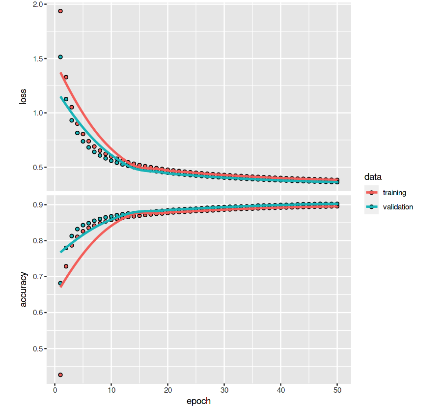
In conclusion, Although the speed and accuracy of the model we implemented above are not better than the packages developed by large manufacturers (such as Tensorflow, Mxnet, etc.), but through step-by-step explanation and coding, it is hoped that interested and novice students can better understand how Softmax regression model solves classification problems and how the mathematical formula behind it is realized. Finally, it is worth mentioning that many people have heard of or used logical regression [logistic regression], in fact, Softmax regression is a broad version of logistic regression. If the classification problem encountered has only two classification objectives (K=2), the hypothesis function and other related formulas of Softmax regression will be simplified into familiar formulas of logistic regression. Interested students can deduce by themselves to see if they can get the formula of logistic regression.