1, Introduction

Histogram of oriented gradient (HOG) is a feature descriptor for target detection in the field of computer vision and image processing. This technique is used to count the number of directional gradients or information in the local image. This method is similar to edge direction histogram, scale invariant feature transformation and shape context method. But the difference between them is that the calculation of hog is based on the density matrix of consistent space to improve the accuracy. That is, it is calculated on a cell with dense grid and uniform size. In order to improve the performance, the overlapping local contrast normalization technology is also used. The combination of hog feature and SVM classifier has been widely used in image recognition, especially in pedestrian detection. This section introduces hog related knowledge.

1 basic introduction

HOG was proposed as a paper published in CVPR by navneet DALAL & bill triggers in 2005 [1]. The author gives the flow chart of feature extraction, as shown in Figure 1:

The core idea of HOG is that the shape of the detected local object can be described by the distribution of light intensity gradient or edge direction. By dividing the whole image into small connected areas called cells, each cell generates a directional gradient histogram or the edge direction of the pixel in the cell. The combination of these histograms can represent the descriptor of the detected target. In order to improve the accuracy, the local histogram can be normalized by calculating the light intensity of a large area called block in the image as a measure, and then normalizing all cells in the block with this measure This normalization process achieves better illumination / shadow invariance. Compared with other descriptors, the descriptors obtained by HOG maintain geometric and optical transformation invariance unless the object direction changes. The relationship between block and cells is shown in the following figure:

Now, we give the pedestrian detection test done by the author, as shown in Figure 6:

Wherein (a) in the figure represents the average gradient of all training image sets; (b) And © Respectively represent: the maximum positive and negative SVM weights on each interval in the image; (d) Represents a test image; (e) Test image after calculating R-HOG; (f) And (g) represent R-HOG images weighted by positive and negative SVM weights, respectively.

3 algorithm description

HOG feature extraction method: firstly, the image is divided into small connected regions, which we call cell units. Then, the direction histogram of the gradient or edge of each pixel in the cell unit is collected. Finally, these histograms can be combined to form a feature descriptor. As shown in the figure below.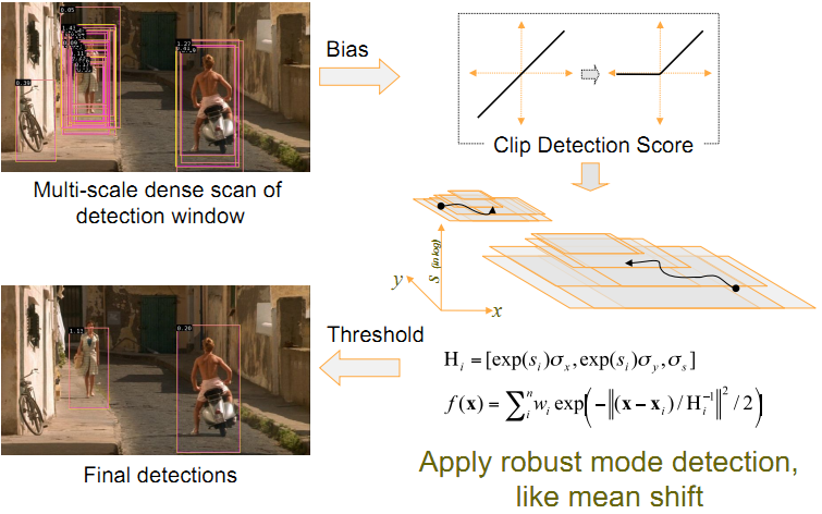

That is: gray an image: the first step is to treat the image as a three-dimensional image of X, y and Z (gray); Step 2: divide into small cells(2*2); Step 3: calculate the gradient (i.e. orientation) of each pixel in each cell; Finally, the gradient histogram of each cell (the number of different gradients) is counted to form the descriptor of each cell. The specific process of the whole algorithm consists of the following parts:

4 color and gamma normalization

In practical application, this step can be omitted because the author normalizes the image color and gamma in gray space, RGB color space and LAB color space respectively. The experimental results show that the normalization preprocessing has no effect on the final results, and there are normalization processes in the subsequent steps, which can replace the normalization of the preprocessing. See reference [1] for details

5 gradient calculation

Simply use a one-dimensional discrete differential template to process the image in one direction or in both horizontal and vertical directions. More specifically, this method needs to use the following filter core to filter out the color or rapidly changing data in the image. The author also tried some other more complex templates, such as 3 × 3 Sobel template, or diagonal masks, but in this pedestrian detection experiment, the performance of these complex templates is poor, so the author's conclusion is that the simpler the template, the better the effect. The author also tried to add a Gaussian smoothing filter before using the differential template, but the addition of this Gaussian smoothing filter makes the detection effect worse. The reason is that many useful image information comes from rapidly changing edges, which will be filtered out by adding Gaussian filter before calculating the gradient.

6 creating the orientation histograms

This step is to construct a gradient direction histogram for each cell unit of the image. Each pixel in the cell cell votes for a direction based histogram channel. Voting adopts the method of weighted voting, that is, each vote is weighted, which is calculated according to the gradient amplitude of the pixel. The amplitude itself or its function can be used to represent the weight. The actual test shows that using the amplitude to represent the weight can obtain the best effect. Of course, the amplitude function can also be selected to represent, such as the square root of the amplitude, the square of the amplitude, the truncation form of the amplitude, etc. Cell units can be rectangular or star shaped. Histogram channels are evenly distributed in the undirected (0180 degrees) or directed (0360 degrees).
It is found that the best effect can be achieved in pedestrian detection experiment by using undirected gradient and 9 histogram channels. The cell units are combined into a large range. Due to the change of local illumination and the change of foreground background contrast, the variation range of gradient intensity is very large. This requires the normalization of gradient intensity. The method adopted by the author is to combine each cell unit into large and spatially connected blocks. Thus, the HOG descriptor becomes a vector composed of histogram components of all cell units in each interval. These intervals overlap each other, which means that the output of each cell unit acts on the final descriptor many times. The interval has two main geometries: rectangular interval (R-HOG) and annular interval (C-HOG).


R-HOG: R-HOG intervals are generally square lattices, which can be characterized by three parameters: the number of cell units in each interval, the number of pixels in each cell unit, and the number of histogram channels of each cell. Experiments show that the best parameter setting of pedestrian detection is: 3 × 3 cells / interval, 6 × 6 pixels / cell, 9 histogram channels. The author also found that it is very necessary to add a Gaussian spatial window to each block before processing the histogram, because it can reduce the weight of pixels around the edge. R-HOG and sift descriptors look very similar, but their differences are: R-HOG is calculated in a single scale, dense grid and no direction sorting; The SIFT descriptor is calculated in the case of multi-scale, sparse image key points and sorting directions. In addition, R-HOG is that each interval is combined to encode airspace information, while each descriptor of sift is used separately.
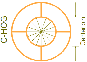
C-HOG: there are two different forms of C-HOG interval. The difference is that a central cell is complete and a central cell is divided. As shown in the figure above, the author found that both forms of C-HOG can achieve the same effect. The C-HOG interval can be characterized by four parameters: the number of angle boxes, the number of radius boxes, the radius of the central box and the extension factor of the radius. Through the experiment, for pedestrian detection, the best parameters are: 4 angle boxes, 2 radius boxes, the radius of the central box is 4 pixels, and the extension factor is 2. As mentioned earlier, it is very necessary to add a Gaussian airspace window in the middle for r-hog, but it is not necessary for C-HOG. C-HOG looks like the method based on Shape Contexts, but the difference is that the cell unit contained in the interval of C-HOG has multiple orientation channels, while the method based on shape context only uses a single edge presence count.

Block normalization schemes the author uses four different methods to normalize the interval, and compares the results. Introduce v to represent a vector that has not been normalized yet, which contains all histogram information of a given block. | vk | represents the k-order norm of v, where k goes to 1 and 2. Use e to represent a small constant. At this time, the normalization factor can be expressed as follows: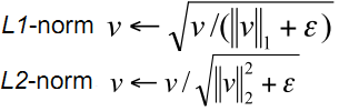

L2 norm: L1 norm: L1 sqrt: there is also a fourth normalization method: L2 HYS, which can be obtained by first performing L2 norm, clipping the results, and then re normalizing. The author found that the effect of using L2 HYS L2 norm and L1 sqrt is the same, and L1 norm shows a little unreliability. However, for the data not normalized, these four methods show significant improvements. The last step of SVM classifier is to input the extracted HOG features into SVM classifier and find an optimal hyperplane as the decision function. The author adopts the method of using free SVMLight software package and HOG classifier to find pedestrians in the test image.
In conclusion, HoG has no rotation and scale invariance, so the amount of calculation is small; Each feature in sift needs to be described by 128 dimensional vectors, so the amount of calculation is relatively large. In pedestrian detection, to solve the problem of scale invariant: scaling the image at different scales is equivalent to scaling the template at different scales To solve the problem of rotation invariant: establish templates in different directions (generally 157) for matching. In general, images on different scales are matched with templates in different directions, and each point forms an 8-direction gradient description. Sift does not need pedestrian detection because of its huge amount of computation, while PCA-SIFT filters out many dimensions of information and retains only 20 principal components, so it is only suitable for object detection with little change in behavior.
Compared with other feature description methods (such as sift, PCA-SIFT, SURF), HOG has the following advantages: firstly, because HOG operates on the local grid unit of the image, it can maintain good invariance to the geometric and optical deformation of the image, and these two deformations will only appear in a larger spatial field. Secondly, under the conditions of coarse spatial sampling, fine directional sampling and strong local optical normalization, as long as pedestrians can generally maintain an upright posture, pedestrians can be allowed to have some subtle limb movements, which can be ignored without affecting the detection effect. Therefore, the HOG feature is particularly suitable for human body detection in images.

2, Partial code

clc
clear all;
close all;
load('AR_HOG')
%Divide training set and test set
% for i=1:1:120
%    eval(['train_',num2str(i),'=','zeros(20,1824)'';']);
%    %train_set = zeros(20*120,1824);
%    %test_set = zeros(6*120,1824);
%    eval(['test_',num2str(i),'=','zeros(6,1824)'';']); 
% for j=1:1:20
%     eval(['train_',num2str(i),'(:,j)','=','my_lbp(:,26*(i-1)+j)'';']);
% end
% for k=1:1:6
%     eval(['test_',num2str(i),'(:,k)','=','my_lbp(:,26*(i-1)+k+20)'';']);
% end
% end
 
%% Data division
train_set = zeros(20*120,720);
test_set = zeros(6*120,720);
 train_set = [];
 test_set = [];
for i = 1:120
     train_set = pic_all(:,(i-1)*26+1:(i-1)*26+20);
     test_set = pic_all(:,(i-1)*26+21:(i-1)*26+26);
end
%% classification
label = zeros(6*120,1);
for i = 1:6*120
    y = test_set(:,i);
    dis = sqrt(sum((train_set - repmat(y,1,20*120)).^2));%Calculate distance
    local = find(dis == min(dis));
    if mod(local,20)~= 0
        label(i) = fix(local/20)+1;
    else 
        label(i) = local/20;
    end
    
end
 
 
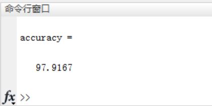
%% Calculation accuracy
a = 1:120;
a = repmat(a,6,1);
real_label = a(:);
dis_label = real_label - label;
acc_rate = length(find(dis_label == 0))/(120*6);
 
 
 
 
 
 
 
%Comparison of absolute distance and Euclidean distance 3
% D=0;D1=1;
% for i=1:1:120
%  for j=1:1:19
%   for k=j+1:1:20
% a=eval(['train_',num2str(i),'(:,j)',';']);
% b=eval(['train_',num2str(i),'(:,k)',';'])';
% d=mandist(b,a);
% D=D+d;
% d1=dist(b,a);
% D1=D1+d1;
%   end
%  end
% eval(['ave_d_',num2str(i),'=','D/190'';']);
% eval(['ave_d1_',num2str(i),'=','D1/190'';']);
% D=0;D1=0;
% end
% o=0;f=0;q=0;w=0;
% for i=1:1:120
%  for j=1:1:6
%   for k=1:1:20
%       a=eval(['train_',num2str(i),'(:,k)',';']);
%       b=eval(['test_',num2str(i),'(:,j)',';'])';
%       d=mandist(b,a);
%       d1=dist(b,a);
%   end
%    if d<=1.1*eval(['ave_d_',num2str(i)])
%     f=f+1;
%    else
%        q=q+1;
%    end
%    if d1<=1.1*eval(['ave_d1_',num2str(i)])
%     o=o+1;
%    else
%        w=w+1;
%    end
function  featureVec= hog(img)
img=double(img);
step=8;  %8*8 Pixels as one cell
[m1 n1]=size(img);
%Change image size to step Nearest integer multiple of
img=imresize(img,[floor(m1/step)*step,floor(n1/step)*step],'nearest');
[m n]=size(img);
% 2,%Gamma correction 
img=sqrt(img);
% 3,Find gradient sum direction
fy=[-1 0 1];        %Define vertical template
fx=fy';             %Define horizontal template
Iy=imfilter(img,fy,'replicate');    %Vertical gradient
Ix=imfilter(img,fx,'replicate');    %Horizontal gradient
Ied=sqrt(Ix.^2+Iy.^2);              %gradient magnitude 
Iphase=Iy./Ix;              %Edge slope, some are inf,-inf,nan，among nan It needs to be dealt with again
the=atan(Iphase)*180/3.14159; %Find gradient angle
 
 
for i=1:m
    for j=1:n
        if(Ix(i,j)>=0&&Iy(i,j)>=0) %first quadrant
            the(i,j)=the(i,j);
        elseif(Ix(i,j)<=0&&Iy(i,j)>=0) %Beta Quadrant 
            the(i,j)=the(i,j)+180;
        elseif(Ix(i,j)<=0&&Iy(i,j)<=0) %third quadrant 
            the(i,j)=the(i,j)+180;
        elseif(Ix(i,j)>=0&&Iy(i,j)<=0) %Delta Quadrant 
            the(i,j)=the(i,j)+360;
        end
        if isnan(the(i,j))==1  %0/0 Will get nan，If the pixel is nan，Reset to 0
            the(i,j)=0;
        end
    end
end
the=the+0.000001; %The prevention angle is
% 4,divide cell，seek cell Histogram of( 1 cell = 8*8 pixel )
%Here's a request cell
step=8;                %step*step Pixels as one cell
orient=9;               %Number of direction histograms
jiao=360/orient;        %Number of angles per direction
Cell=cell(1,1);              %All angle histograms,cell It can be added dynamically, so set one first
ii=1;
jj=1;
for i=1:step:m
    ii=1;
    for j=1:step:n
        Hist1(1:orient)=0;
        for p=1:step
            for q=1:step
                %Gradient direction histogram
                Hist1(ceil(the(i+p-1,j+q-1)/jiao))=Hist1(ceil(the(i+p-1,j+q-1)/jiao))+Ied(i+p-1,j+q-1);
            end
        end
        Cell{ii,jj}=Hist1;       %Put Cell in
        ii=ii+1;
    end
    jj=jj+1;
end
% 5,divide block，seek block Eigenvalue of,Use overlap( 1 block = 2*2 cell )
[m n]=size(Cell);
feature=cell(1,(m-1)*(n-1));
for i=1:m-1
    for j=1:n-1
        block=[];
        block=[Cell{i,j}(:)' Cell{i,j+1}(:)' Cell{i+1,j}(:)' Cell{i+1,j+1}(:)'];
        block=block./sum(block); %normalization
        feature{(i-1)*(n-1)+j}=block;
    end
end
% 6,Pictorial HOG characteristic value
[m n]=size(feature);
l=2*2*orient;
featureVec=zeros(1,n*l);
for i=1:n
    featureVec((i-1)*l+1:i*l)=feature{i}(:);
end
%  [m n]=size(img);
%  img=sqrt(img);      %Gamma correction 
% %The following is to find the edge
% fy=[-1 0 1];        %Define vertical template
% fx=fy';             %Define horizontal template
% Iy=imfilter(img,fy,'replicate');    %Vertical edge
% Ix=imfilter(img,fx,'replicate');    %Horizontal edge
% Ied=sqrt(Ix.^2+Iy.^2);              %Edge strength
% Iphase=Iy./Ix;              %Edge slope, some are inf,-inf,nan，among nan It needs to be dealt with again
% 
% 
% %Here's a request cell
% step=16;                %step*step Pixels as a unit
% orient=9;               %Number of direction histograms
% jiao=360/orient;        %Number of angles per direction
% Cell=cell(1,1);              %All angle histograms,cell It can be added dynamically, so set one first
% ii=1;                      
% jj=1;
% for i=1:step:m          %If handled m/step Not an integer, preferably i=1:step:m-step
%     ii=1;
%     for j=1:step:n      %Ibid
%          tmpx=Ix(i:i+step-1,j:j+step-1);
%         tmped=Ied(i:i+step-1,j:j+step-1);
%         tmped=tmped/sum(sum(tmped));        %Local edge intensity normalization
%         tmpphase=Iphase(i:i+step-1,j:j+step-1);
%         Hist=zeros(1,orient);               %current step*step Pixel block statistical angle histogram,namely cell
%         for p=1:step
%             for q=1:step
%                 if isnan(tmpphase(p,q))==1  %0/0 Will get nan，If the pixel is nan，Reset to 0
%                     tmpphase(p,q)=0;
%                 end
%                 ang=atan(tmpphase(p,q));    %atan What I'm asking is[-90 90]Between degrees
%                 ang=mod(ang*180/pi,360);    %All positive,-90 Change 270
%                 if tmpx(p,q)<0              %according to x Direction determines the true angle
%                     if ang<90               %If it's the first quadrant
%                         ang=ang+180;        %Move to the third quadrant
%                     end
%                     if ang>270              %If it's the fourth quadrant
%                         ang=ang-180;        %Move to the second quadrant
%                     end
%                 end
%                 ang=ang+0.0000001;          %prevent ang Is 0
%                 Hist(ceil(ang/jiao))=Hist(ceil(ang/jiao))+tmped(p,q);   %ceil Round up using edge strength weighting
%             end
%         end

3, Operation results