Original link: http://tecdat.cn/?p=24973
Original source: Tuo end data tribal official account
brief introduction
The World Health Organization estimates that 12 million people worldwide die of heart disease every year. In the United States and other developed countries, half of the deaths are due to cardiovascular disease. The early prognosis of cardiovascular disease can help decide to change the lifestyle of high-risk patients, so as to reduce complications. The purpose of this study was to identify the most relevant / risk factors for heart disease and use machine learning to predict the overall risk.
Data preparation
source
The data set comes from an ongoing cardiovascular study of residents. The classification goal is to predict whether patients will have the risk of coronary heart disease (CHD) in the next 10 years. Data sets provide patient information. It includes more than 4000 records and 15 attributes.
variable
Each attribute is a potential risk factor. There are demographic, behavioral and medical risk factors.
Demographics:
• gender: male or female (scalar)
• age: patient age; (continuous - although the recorded age has been truncated to an integer, the concept of age is continuous)
behavior
• current smoker: is the patient a current smoker (scalar)
• number of cigarettes smoked per day: the average number of cigarettes smoked by this person in a day. (it can be considered continuous, because a person can have any number of cigarettes, or even half a cigarette.)
• BP Meds: does the patient take antihypertensive drugs (scalar)
• stroke: did the patient have a previous stroke (scalar)
• Hyp: does the patient have hypertension (scalar)
Diabetes: does the patient have diabetes (scalar)?
• Tot Chol: total cholesterol level (continuous)
• Sys BP: systolic blood pressure (continuous)
• Dia BP: diastolic blood pressure (continuous)
• BMI: body mass index (continuous)
• heart rate: heart rate (continuous - in medical research, although variables such as heart rate are actually discrete, they are considered continuous due to the existence of a large number of possible values.)
• glucose: glucose level (continuous)
Predictive variables (expected objectives)
• 10-year risk of CHD (binary: "1" for "yes", "0" for "no")
Heart disease prediction
# get data
rdaa <- read.csv((path)
# Here, we can consider increasing the difference between systolic blood pressure and diastolic blood pressure, and describing the variables of systolic blood pressure, diastolic blood pressure and hypertension level

# Look at the data structure
str(ata)
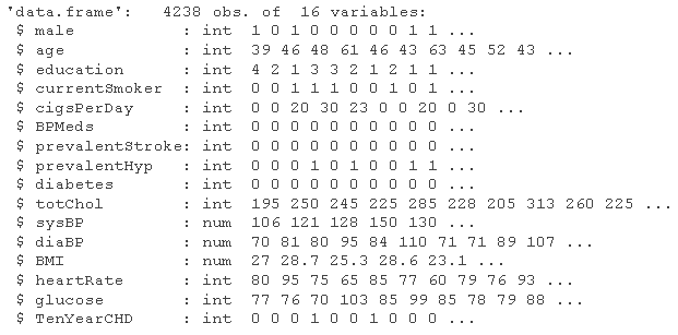
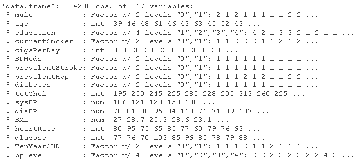
# Consider adding the variable bplevel
raw_data <- sqldf

# Distinguish between variable categories

ra_da <- map
str(ra_da )
Data preprocessing
Viewing and processing missing values
# Here we use the Mie package to handle missing values
aggr
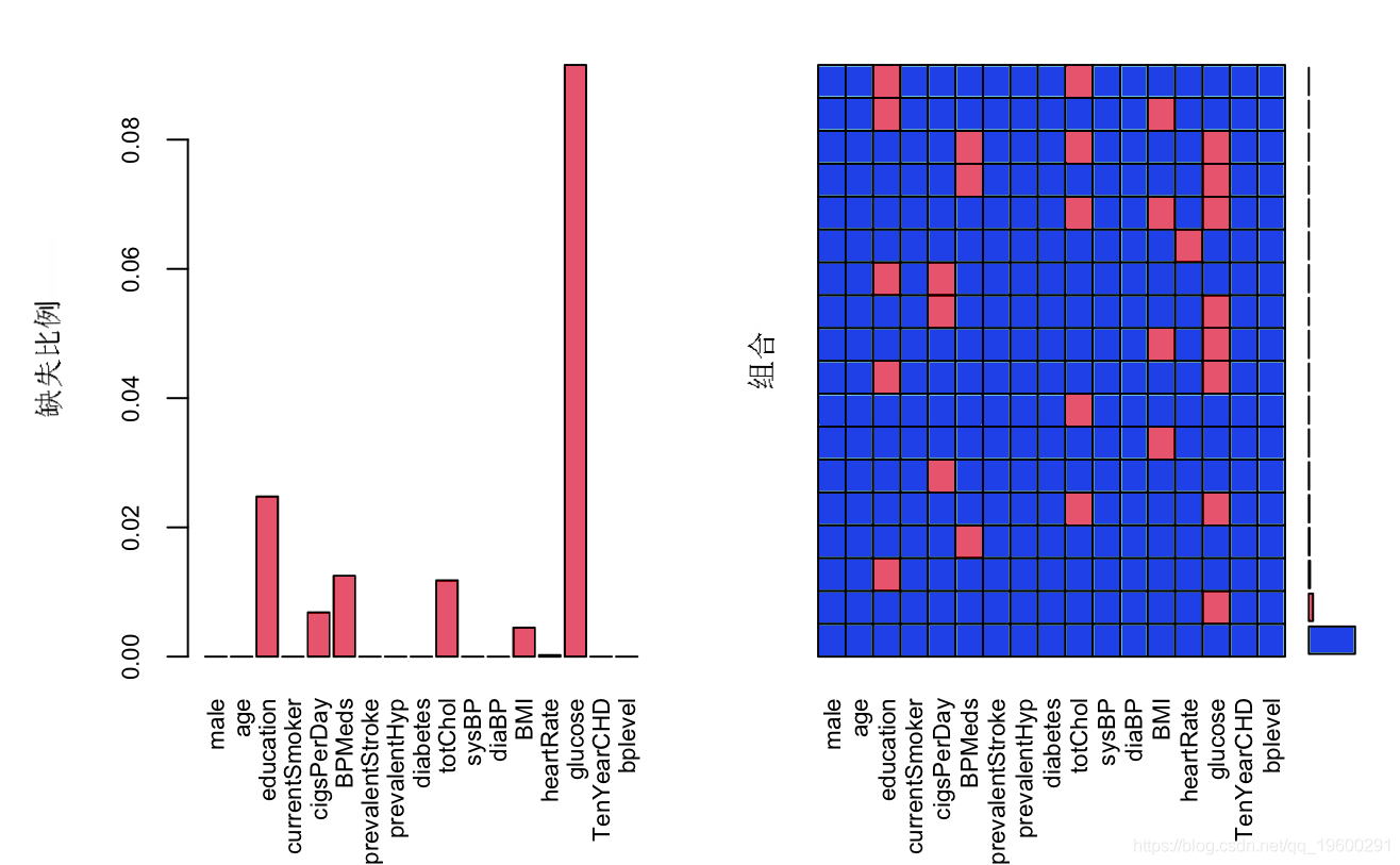
matplot
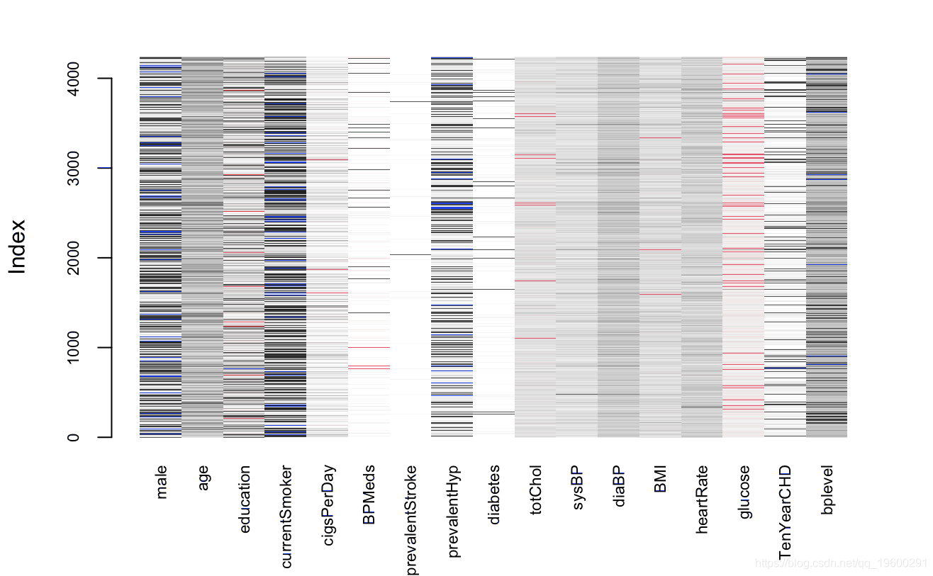
As can be seen from the above figure, except for the glucose variable, the deletion proportion of other variables is less than 5%, and the deletion rate of glucose variable is more than 10%. The processing strategy is to keep the missing value of glucose variable and directly delete the missing value of other variables. Now deal with the missing value of glucose,
# Processing glucose columns
lee_a <- subset & !is.na & !is.na & !is.na & !is.na & !is.na
# Check the linear correlation between glce and other variables to determine the filling strategy of mice
gcog = glm(lcse ~ .)
smry(glseg)
Fill in and exclude unimportant variables. As for why diaBP is not selected, it is mainly because these two variables will cause multicollinearity in the later correlation analysis.
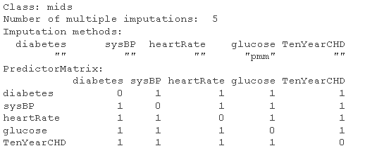
mice%in%  m=5,  "pmm", mai = 50, sd=2333, pint= FALSE)
#View fill results
smr(mc_od)
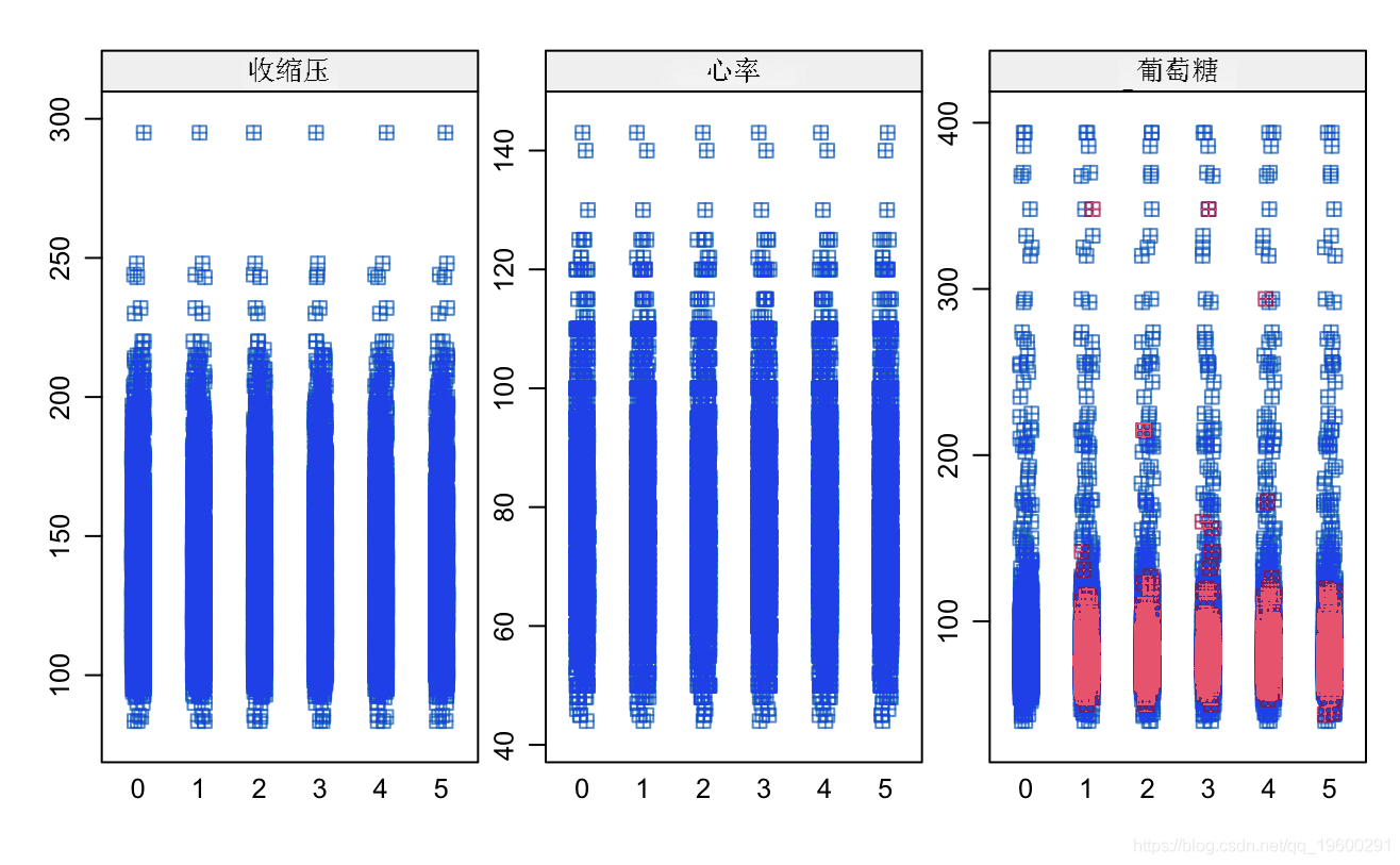
# View the distribution of original data and interpolated data
epot(mi_md)
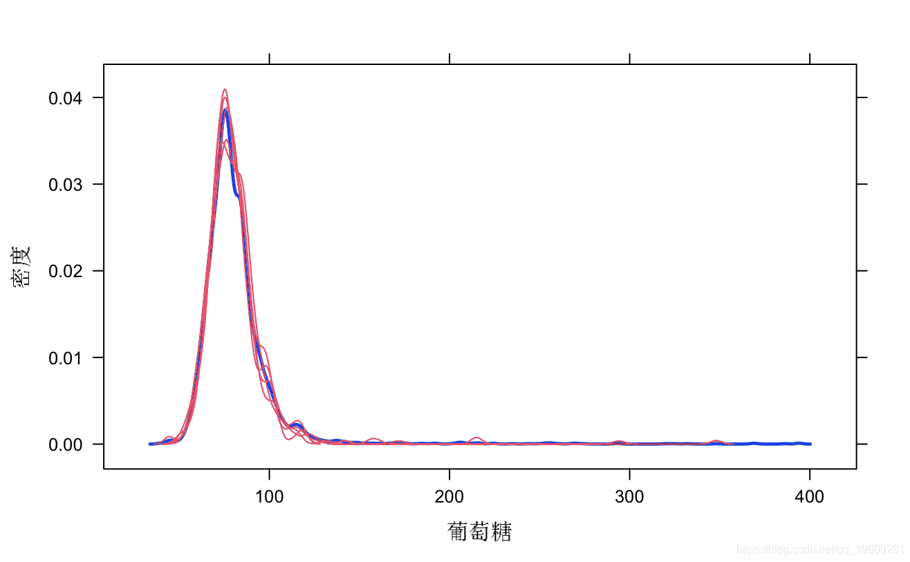
sipt(mcod, pch=12)
# Fill data
mi_t <- complete
fir_aa$loe <- miout$guose
sum(is.na(flda))

Delete duplicate lines
# Check for duplicate lines and delete duplicate lines
sum(duplicated

comd_ata <- comdta[!duplicated(), ]
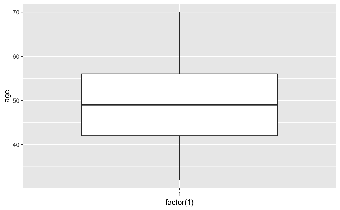
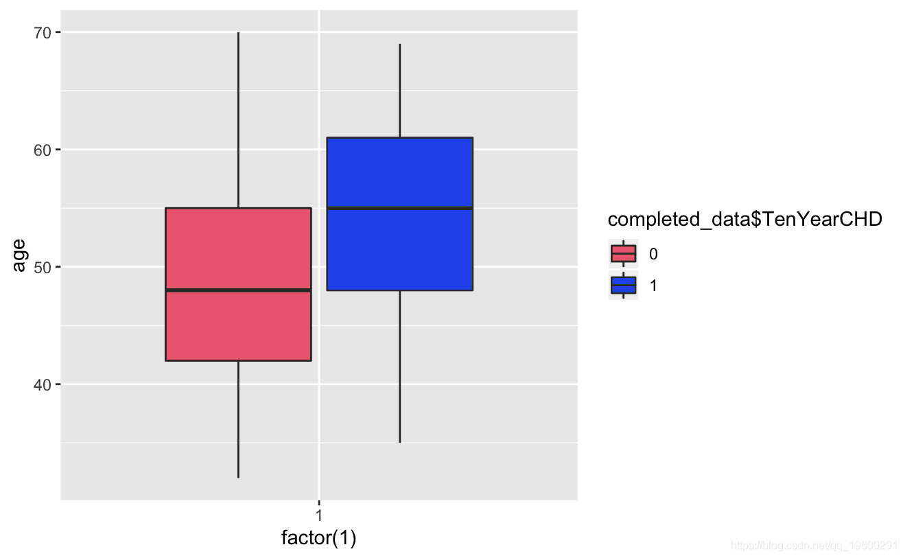
View outliers
#View outliers
gplot(coedta)+geom_boxplot(ae(ftr(1),age))
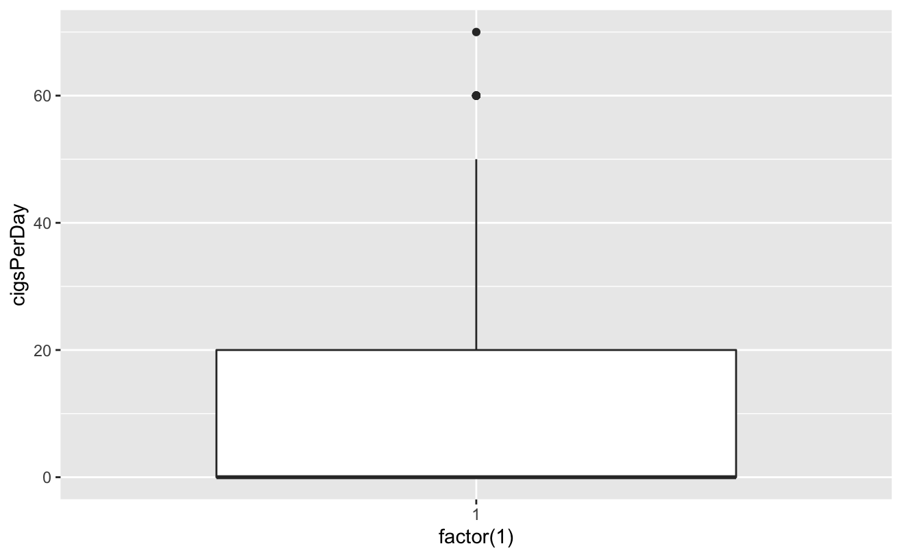
ggplot(copd_dta)+geom_boxplot(aes(factor(1cigDy))
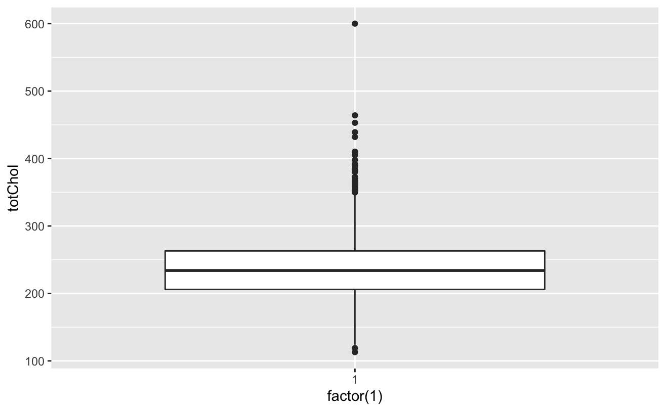
ggplot(coea)+geom_boxplot(aes(factor(1),ttl))
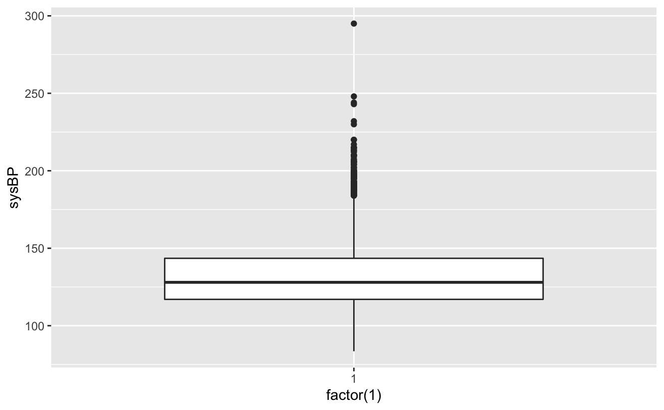
ggplot(colt_ta)+geom_boxplot(aes(factor(1),syBP))
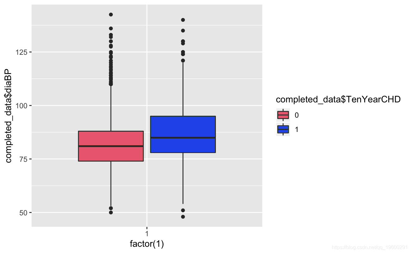
ggplot(comeaa)+geom_boxplot(aes(factor(1),daP))
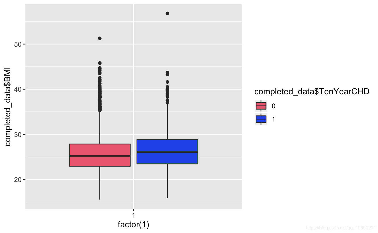
ggplot()+gem_boxplot(aes(factor(1),BMI))
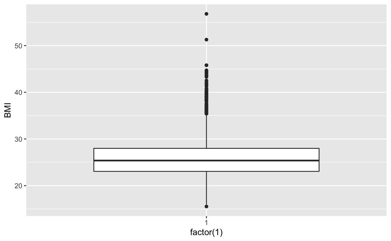
# View cigsPerDay
cigs_sub <- comled_dta
# View tothol and delete outliers
# View sysBP and delete outliers
# View BMI
totChol: the total cholesterol level greater than 240mg/dl is very high, so the record with the level of 600mg/dl is deleted. sysBP: remove the record of systolic blood pressure of 295mg/dl
# Delete outliers of each variable
competedata
# Categorical variable contingency analysis
ggplot+geom_boxplot
ggplot+geom_boxplot(aes,totChol,fill=TenYerCHD))
cometddata %>% fitr %>%
ggplot
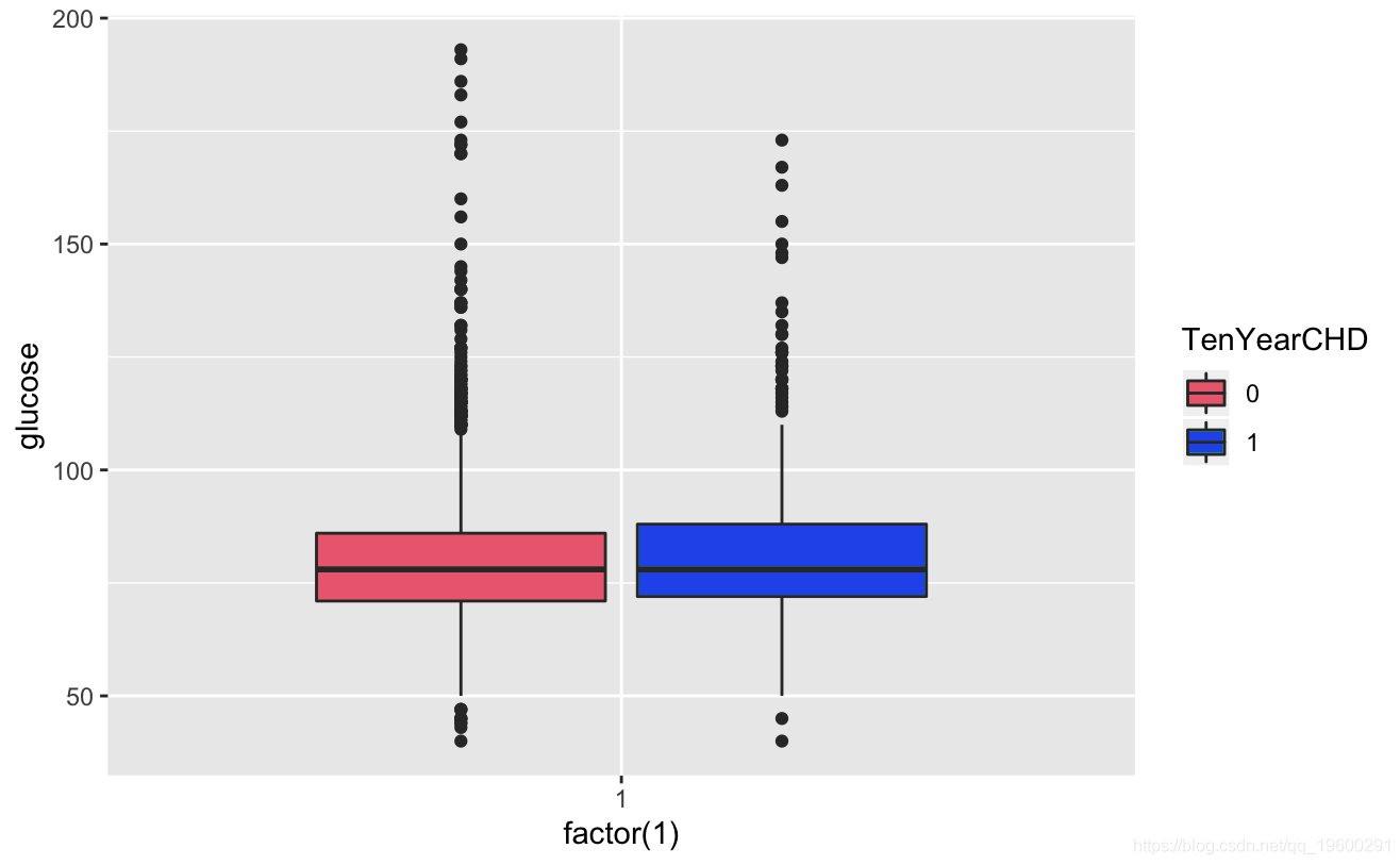


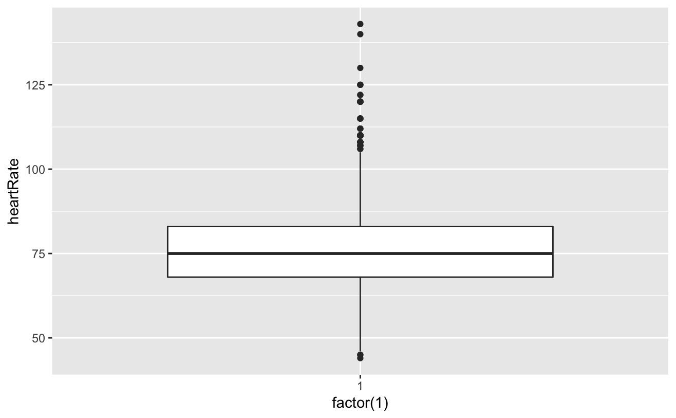
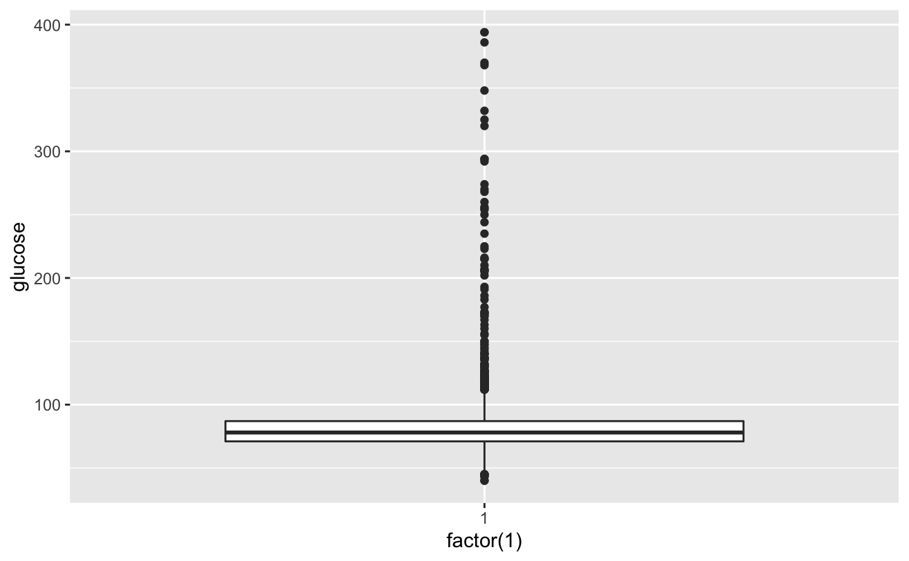
Known from the image, the glucose and hearRate variables have no significant risk
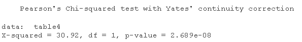
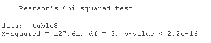
table1=table
chisq.test
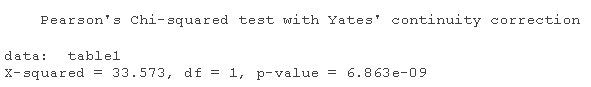
table1
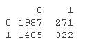
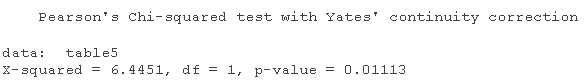
table2=table
chisq.test
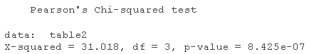
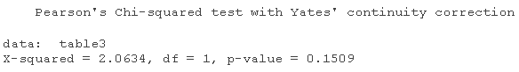
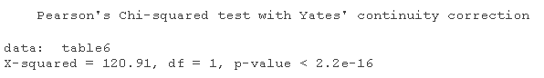
table3=table
chisq.test
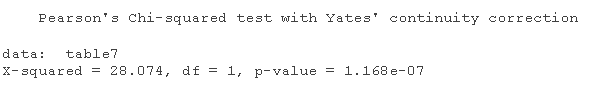
chisq.test
ggpairs

diaBP and sysBP have multicollinearity problems.
The currentSmoker variable may not be significant, so go to the model section below.
Model
# Partition dataset

split = sample.split

train = subset
logistic regression
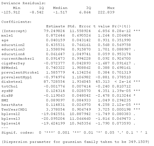
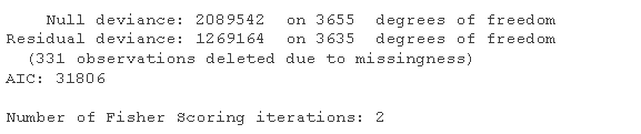
# Logistic regression model - use all variables
fultaog = glm
summary(fulog)
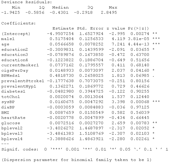
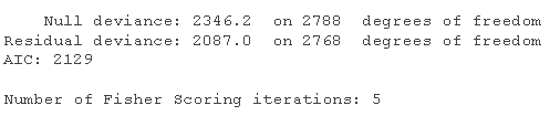
fldaog = glm
summary(fuatLg)
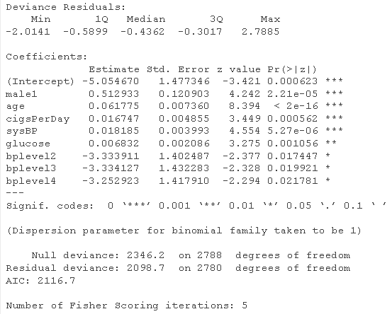
prdts = predict
glm_le <- table
ACCU

Random forest
rfoel <- randomForest
# Gain importance
imprace
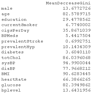
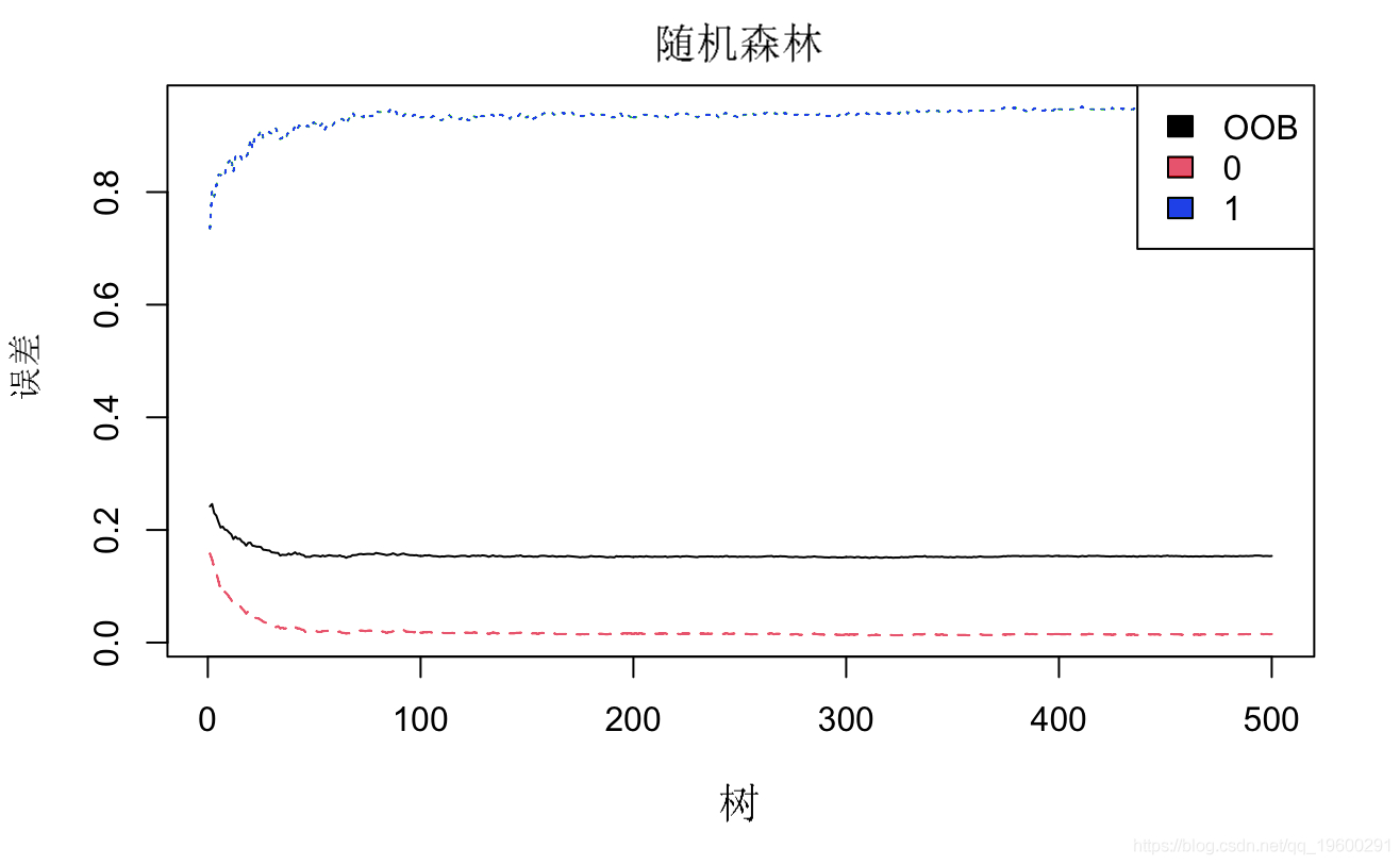
# Select important factors
rfmdel <- randomForest
# error
plot
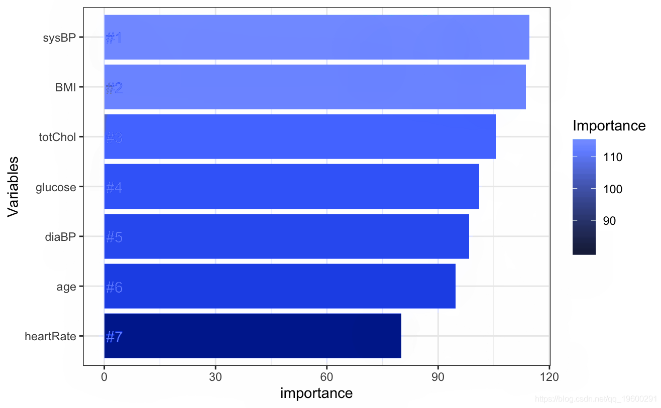
# Acquisition importance
ggplot +
   geom_bar
   geom_text
There is an error in the risk of disease, which does not decrease but increases. We need to explore the reasons
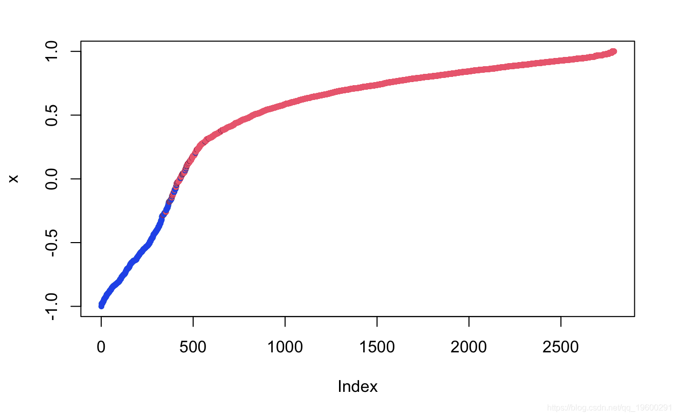
# Draw classified image
pred<-predict
pdou_1<-predict  #Output probability
table <- table
sum(diag/sum #Prediction accuracy

plot(margin
support vector machines
# Model tuning first
tud <- tune.svm
summary(tud )
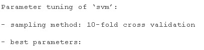
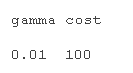
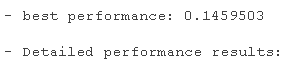

# Using turning function to get the best parameter setting support vector machine
mel.nd <- svm
cost=tuned$
summary(modted)
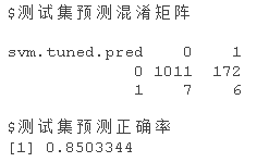
# Call the predict function to predict the class label based on the newly configured SVM model:
sm.ne.ed <- predict
sv.tuedtble <- table
sm.ue.tbe
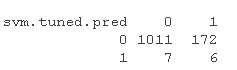
acy.s.vm <- sum(diag)/sum
Model diagnosis
According to the results of the above three models, it can be seen that the distribution of category number of prediction results is very uneven
sum

sum(TeYaHD == 0)

In view of this phenomenon, methods need to be taken to balance the data set.

Most popular insights
1.Application case of multiple Logistic regression in R language
2.Implementation of panel smooth transfer regression (PSTR) analysis case
3.Partial least squares regression (PLSR) and principal component regression (PCR) in matlab
4.Case study of Poisson Poisson regression model in R language
5.R language mixed effect Logistic regression model analysis of lung cancer
6.Implementation of LASSO regression, Ridge ridge regression and Elastic Net model in r language