Opencv -- image processing

Grayscale image output:

import cv2 #The format read by opencv is BGR
import numpy as np
import matplotlib.pyplot as plt#Matplotlib is RGB
%matplotlib inline 

img=cv2.imread('miku.png')
img_gray = cv2.cvtColor(img,cv2.COLOR_BGR2GRAY)
img_gray.shape

cv2.imshow("img_gray", img_gray)
cv2.waitKey(0)    
cv2.destroyAllWindows()

Picture output:

Convert BGR format pictures to HSV format, where:

HSV

H - hue (dominant wavelength).
S - saturation (purity / shade of color).
V value (strength)

hsv=cv2.cvtColor(img,cv2.COLOR_BGR2HSV)

cv2.imshow("hsv", hsv)
cv2.waitKey(0)    
cv2.destroyAllWindows()

Picture output:

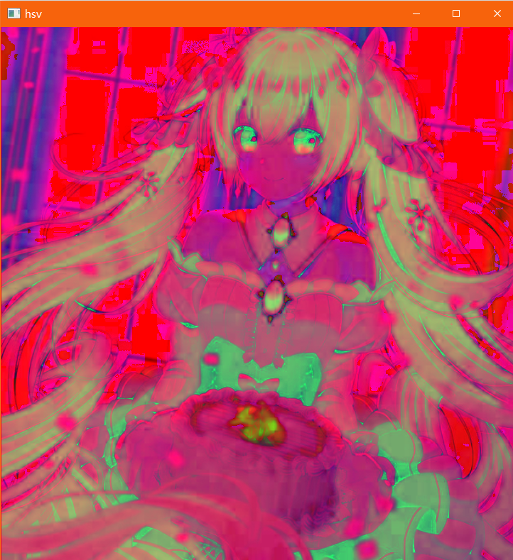
Image threshold:

We know that each picture is composed of a large number of different pixels. The pixel illumination range is 0-255. The threshold operation is to specify the threshold of the pixels that meet the range. For example, all pixels higher than 127 are uniformly set to 255, which is a highlight function_ INV is reverse operation.

ret, dst = cv2.threshold(src, thresh, maxval, type)

src: input image, only single channel image can be input, usually gray image
dst: output diagram
thresh: threshold
maxval: the value assigned when the pixel value exceeds the threshold (or is less than the threshold, depending on the type)
Type: the type of binarization operation, including the following five types: CV2 THRESH_ BINARY； cv2.THRESH_BINARY_INV； cv2.THRESH_TRUNC； cv2.THRESH_TOZERO； cv2.THRESH_TOZERO_INV
cv2. THRESH_ If binary exceeds the threshold value, take maxval (maximum value), otherwise take 0
cv2. THRESH_ BINARY_ INV THRESH_ Inversion of binary
cv2. THRESH_ The part of TRUNC greater than the threshold value is set as the threshold value, otherwise it remains unchanged
cv2. THRESH_ The part where tozero is greater than the threshold does not change, otherwise it is set to 0
cv2. THRESH_ TOZERO_ INV THRESH_ Inversion of tozero

ret, thresh1 = cv2.threshold(img_gray, 127, 255, cv2.THRESH_BINARY)
ret, thresh2 = cv2.threshold(img_gray, 127, 255, cv2.THRESH_BINARY_INV)
ret, thresh3 = cv2.threshold(img_gray, 127, 255, cv2.THRESH_TRUNC)
ret, thresh4 = cv2.threshold(img_gray, 127, 255, cv2.THRESH_TOZERO)
ret, thresh5 = cv2.threshold(img_gray, 127, 255, cv2.THRESH_TOZERO_INV)

titles = ['Original Image', 'BINARY', 'BINARY_INV', 'TRUNC', 'TOZERO', 'TOZERO_INV']
images = [img, thresh1, thresh2, thresh3, thresh4, thresh5]
                                 
for i in range(6):
    plt.subplot(2, 3, i + 1), plt.imshow(images[i], 'gray')
    plt.title(titles[i])
    plt.xticks([]), plt.yticks([])
plt.show()

Picture output:

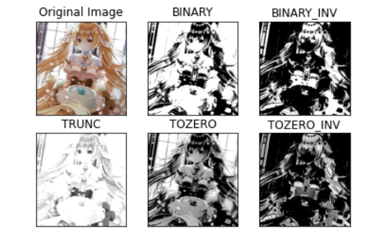
As can be seen from the figure, the black-and-white contrast is relatively high, while_ INV is reverse operation.

Image smoothing:

Some noise points may appear in some pictures. At this time, we need to filter and smooth the noise points.

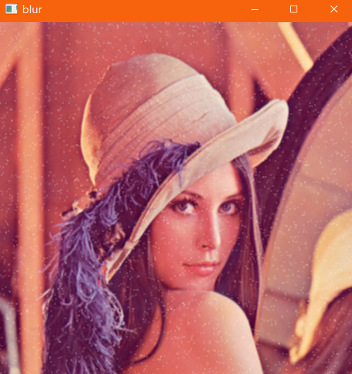
Mean filtering:

# Mean filtering
# Simple average convolution operation
blur = cv2.blur(img, (3, 3))

cv2.imshow('blur', blur)
cv2.waitKey(0)
cv2.destroyAllWindows()

effect:

Box filtering: essentially, it is similar to the mean value. After normalization, it is the mean value filtering. Note that without normalization, there may be overflow and exposure

# box filter 
# Basically the same as the mean, normalization can be selected
box = cv2.boxFilter(img,-1,(3,3), normalize=True)  

cv2.imshow('box', box)
cv2.waitKey(0)
cv2.destroyAllWindows()

# box filter 
# Basically the same as the mean value, normalization can be selected, which is easy to cross the boundary
box = cv2.boxFilter(img,-1,(3,3), normalize=False)  

cv2.imshow('box', box)
cv2.waitKey(0)
cv2.destroyAllWindows()

Effect: there is almost no difference between normalization and mean value in Figure 1, and a large number of pixels in Figure 2 are out of bounds.

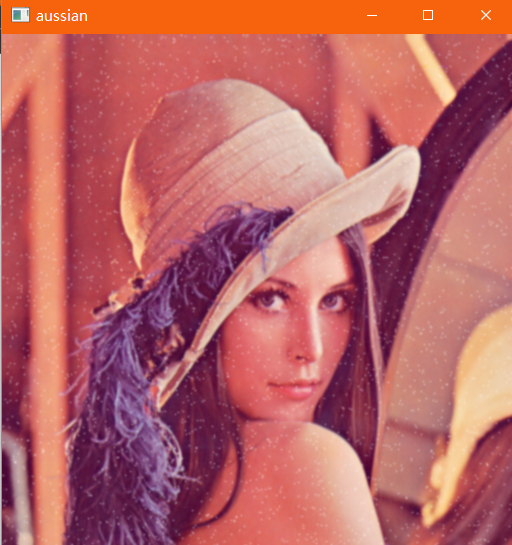
Gaussian filtering:

# Gaussian filtering
# The value in the convolution kernel of Gaussian blur satisfies the Gaussian distribution, which is equivalent to paying more attention to the middle
aussian = cv2.GaussianBlur(img, (5, 5), 1)  

cv2.imshow('aussian', aussian)
cv2.waitKey(0)
cv2.destroyAllWindows()

effect:

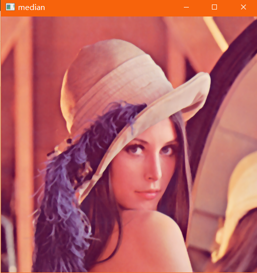
Median filter: replace with median, which is equivalent to directly ignoring noise points, and the effect is the best

# median filtering 
# Equivalent to replacing with median
median = cv2.medianBlur(img, 5)  # median filtering 

cv2.imshow('median', median)
cv2.waitKey(0)
cv2.destroyAllWindows()

Effect: