In fact, most of the progress in image classification can be attributed to the improvement of training process, such as the increase of data and the change of optimization methods. However, most improvements are not described in detail. Therefore, the authors test and implement these improved methods in this paper, and evaluate the impact of these Tricks on the accuracy of the final model through ablation experiments. By combining these improvements, the author improves various CNN models at the same time. Improve the Top-1 verification accuracy of ResNet-50 from 75.3% to 79.29% on ImageNet. At the same time, it will be proved that improving the accuracy of image classification can also bring better transfer learning performance in other application fields, such as target detection and semantic segmentation.
1,Introduction
In recent years, the list of ImageNet has been refreshed, from Alex net in 2012 to VGg net, NiN, Inception, ResNet, DenseNet and NASNet; The accuracy of Top-1 also ranges from 62.5% (AlexNet) - > 82.7% (NASNet-a); However, the improvement of such precision is not entirely caused by the change of model architecture, in which the training process will also play a great role, such as the improvement of loss function, the change of data preprocessing mode, and the selection of optimization methods; But this is also an easily overlooked part, so this article will also focus on this issue here.
Table 1 shows the calculation cost and verification accuracy of various models and the training results of ResNet using "Tricks", which can surpass the framework of training using pipeline.
At the same time, it is proved that these Tricks are also effective in other models, such as Inception-V3, MobileNet and so on.
2,Efficient Training
In recent years, hardware has developed rapidly, especially GPU. Therefore, the best choice of many performance related tradeoffs will also change. For example, use lower numerical accuracy and larger batches in training_ Size is more effective.
In this section, various techniques to realize low-precision and large-scale batch training without sacrificing model accuracy are described. Some techniques can even improve accuracy and training speed.
2.1,Large-batch training
Mini batch SGD groups multiple samples into a small batch to increase parallelism and reduce transmission costs. However, using large batch size may slow down your training. For convex optimization problems, the convergence rate decreases with the increase of batch size. Similar empirical conclusions have been published.
In other words, under the same number of epoch s, the training using large batch size will reduce the verification accuracy of the model compared with the training using smaller batches. Many studies have proposed heuristic search methods to solve this problem. Next, we will study four heuristic methods to expand the scale of batch size in single machine training.
1)Linear scaling learning rate
In mini batch SGD, because the samples are randomly selected, gradient descent is also a random process. Increasing the batch size will not change the expectation of random gradient, but will reduce the variance of random gradient. In other words, the noise in the gradient is reduced in large quantities, so we can make greater progress in the opposite direction of the gradient by improving the learning rate.
Goyal et al. Proposed that for ResNet-50 training, the learning rate can be increased linearly according to the batch size empirically. In particular, if 0.1 is selected as the initial learning rate of batch size 256, the initial learning rate can be increased to:
2)Learning rate Warmup
At the beginning of training, all parameters are usually random values, so they are far from the optimal solution. Using an excessive learning rate can lead to numerical instability. In Warmup, a relatively small learning rate is used at the beginning, and then when the training process is stable, it switches back to the initially set learning rate_ lr.
Goyal et al. Proposed a granular warming strategy to linearly increase the learning rate from 0 to the initial learning rate. In other words, assuming that the first m batches (e.g. 5 data epoch) will be used for Warmup, and the initial learning rate is, the learning rate is set to i=m in the first batch.
3)Zero
A ResNet network is composed of multiple residual blocks, and each residual Block is composed of multiple convolution layers. Given the input, assuming that it is the output of the Last Layer, this residual Block will be output. Note that the Last Layer of the Block can be the batch standardization layer.
The BN layer first standardizes its input representation, and then performs a scale transformation. Both parameters and are learnable, and their elements are initialized to 1s and 0s respectively. In the zero initialization heuristic, all BN layers at the end of the remaining blocks are initialized. Therefore, all residual blocks only return their inputs, the number of simulated network layers is less, and it is easier to train in the initial stage.
4)No bias decay
Weight attenuation is usually applied to all learnable parameters, including weights and deviations. It is equivalent to applying L2 regularization to all parameters to make their values close to 0. However, as pointed out by Jia et al., it is recommended to regularize only the weights to avoid over fitting. The unbiased attenuation heuristic follows this recommendation. It only applies the weight attenuation to the weights in the convolution layer and the full connectivity layer. Other parameters, including deviation sum and BN layer, are not regularized.
LARS provides a hierarchical adaptive learning rate and is effective for large batch sizes (over 16K). In the case of single machine training in this paper, the batch size of no more than 2K will usually lead to good system efficiency.
2.2,Low-precision training
Neural networks are usually trained with 32-bit floating-point (FP32) accuracy. In other words, all numbers are stored in FP32 format, and the input, output and calculation operations are participated in by FP32 type. However, the new hardware may have enhanced new arithmetic logic units for lower precision data types.
For example, the Nvidia V100 mentioned earlier provides 14 TFLOPS in FP32 and more than 100 TFLOPS in FP16. As shown in the following table, after switching from FP32 to FP16 on V100, the overall training speed is increased by 2 to 3 times. Despite the performance benefits, the reduced accuracy has a narrower range, making the results more likely to go beyond the range and then interfere with the progress of training. Micikevicius et al proposed storing all parameters and activation in FP16 and calculating the gradient using FP16. At the same time, all parameters in FP32 have a copy for parameter update. In addition, multiplying the loss value by a smaller scalar scaler to better align the accuracy range to FP16 is also a practical solution.
2.3,Experiment Results

3,Model Tweaks
Model adjustment is a small adjustment to the network architecture, such as changing the stripe of a specific volume layer. Such adjustment usually does not change the computational complexity, but may have a non negligible impact on the accuracy of the model.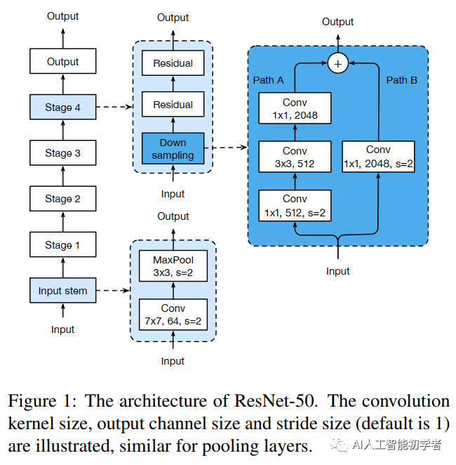
3.1,ResNet Tweaks
Two popular improvements of ResNet, called ResNet-B and ResNet-C, are reviewed. On this basis, a new model adjustment method ResNet-D is proposed.
 1)ResNet-B
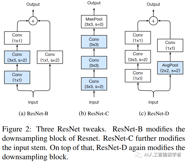
ResNet-B changes the down sampling block. It is observed that the convolution in path a ignores three quarters of the input feature map because it uses a kernel size of 1 × 1. Strike is 2. ResNet-B switches the step size of the first two convolutions in path a, as shown in figure a, so no information is ignored. Because the kernel size of the second convolution is 3 × 3. The output shape of path a remains unchanged.
2)ResNet-C
The computational cost of convolution is the quadratic term of the width or height of the convolution kernel. A 7 × Convolution ratio of 7 3 × The convolution of 3 requires more computation. Therefore, three 3x3 convolutions are used to replace one 7x7 convolution. As shown in Figure b, the channel=32 and stripe = 2 of the first and second convolution block s, and the last convolution uses 64 output channels.
3)ResNet-D
Inspired by ResNet-B, the 1x1 convolution on the path of lower sampling block B also ignores 3 / 4 of the input feature map. Therefore, we want to modify it so that no information will be ignored. Through experiments, it is found that adding an AVG pool layer with an average of 2x2 before convolution and changing its stripe to 1 has a good effect in practice and has little impact on the computational cost.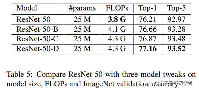
4,Training Refinements
4.1,Cosine Learning Rate Decay
Loshchilov et al. Proposed a cosine annealing strategy. A simplified method is to reduce the learning rate from the initial value to 0 by following the cosine function. Assuming that the total number of batches is t (ignoring the preheating stage), when batch T, the learning rate tm is calculated as:

It can be seen that cosine attenuation slowly reduces the learning rate at the beginning, then almost linearly decreases in the middle and slows down again at the end. Compared with step attenuation, cosine attenuation attenuates learning from the beginning, but continues until step attenuation reduces the learning rate by 10 times, which potentially improves the training progress.
import torch

optim = torch.optim.lr_scheduler.CosineAnnealingLR(optimizer, T_max, eta_min=0, last_epoch=-1)
4.2,Label Smoothing
The output predicted label cannot be as true as the true label. Therefore, a certain smoothing strategy is carried out here. The specific Label Smoothing smoothing rules are as follows:

# -*- coding: utf-8 -*-

"""
qi=1-smoothing(if i=y)
qi=smoothing / (self.size - 1) (otherwise)#So by default, you can fill this number, and only execute 1-smoothing where i=y
 in addition KLDivLoss and crossentroy The difference is that the former has a constant
predict = torch.FloatTensor([[0, 0.2, 0.7, 0.1, 0],

                                 [0, 0.9, 0.2, 0.1, 0],

                                 [1, 0.2, 0.7, 0.1, 0]])
Corresponding label by
tensor([[ 0.0250,  0.0250,  0.9000,  0.0250,  0.0250],
        [ 0.9000,  0.0250,  0.0250,  0.0250,  0.0250],
        [ 0.0250,  0.0250,  0.0250,  0.9000,  0.0250]])
Different from one-hot of
tensor([[ 0.,  0.,  1.,  0.,  0.],
        [ 1.,  0.,  0.,  0.,  0.],
        [ 0.,  1.,  0.,  0.,  0.]])
"""
import torch
import torch.nn as nn
from torch.autograd import Variable
import matplotlib.pyplot as plt
import numpy as np

class LabelSmoothing(nn.Module):
    "Implement label smoothing.  size Indicates the total number of categories  "

    def __init__(self, size, smoothing=0.0):
        super(LabelSmoothing, self).__init__()
        self.criterion = nn.KLDivLoss(size_average=False)
        #self.padding_idx = padding_idx
        self.confidence = 1.0 - smoothing#if i=y
        self.smoothing = smoothing
        self.size = size
        self.true_dist = None

    def forward(self, x, target):
        """
        x Indicates input (N,M)N Samples, M Represents the total number of classes and the probability of each class log P
        target express label(M,)
        """
        assert x.size(1) == self.size
        true_dist = x.data.clone()#Copy it first
        #print true_dist
        true_dist.fill_(self.smoothing / (self.size - 1))#otherwise formula
        #print true_dist
        #Become one hot code, 1 means fill by column,
        #target.data.unsqueeze(1) represents the index, and confidence represents the filled number
        true_dist.scatter_(1, target.data.unsqueeze(1), self.confidence)
        self.true_dist = true_dist
        return self.criterion(x, Variable(true_dist, requires_grad=False))

if __name__=="__main__":
# Example of label smoothing.

    crit = LabelSmoothing(size=5,smoothing= 0.1)
    #predict.shape 3 5
    predict = torch.FloatTensor([[0, 0.2, 0.7, 0.1, 0],
                                 [0, 0.9, 0.2, 0.1, 0],
                                 [1, 0.2, 0.7, 0.1, 0]])

    v = crit(Variable(predict.log()),
             Variable(torch.LongTensor([2, 1, 0])))
    # Show the target distributions expected by the system.
    plt.imshow(crit.true_dist)
4.3,Knowledge Distillation
In the training process, a distillation loss is added to punish the difference between the softmax output of Teacher model and Student model. Given an input, let p be the true probability distribution, and z and r be the output of the last fully connected layer of the Student model and the Teacher model, respectively. The loss is improved to:
4.4,Mixup Training
In Mixup, each time we randomly take two examples and. Then, weighted linear interpolation is performed on the two samples to obtain a new sample:
among
import numpy as np
import torch


def mixup_data(x, y, alpha=1.0, use_cuda=True):
    if alpha > 0.:
        lam = np.random.beta(alpha, alpha)
    else:
        lam = 1.
    batch_size = x.size()[0]
    if use_cuda:
        index = torch.randperm(batch_size).cuda()
    else:
        index = torch.randperm(batch_size)

    mixed_x = lam * x + (1 - lam) * x[index,:] #Superimpose yourself with the disrupted yourself
    y_a, y_b = y, y[index]
    return mixed_x, y_a, y_b, lam

def mixup_criterion(y_a, y_b, lam):
    return lambda criterion, pred: lam * criterion(pred, y_a) + (1 - lam) * criterion(pred, y_b)
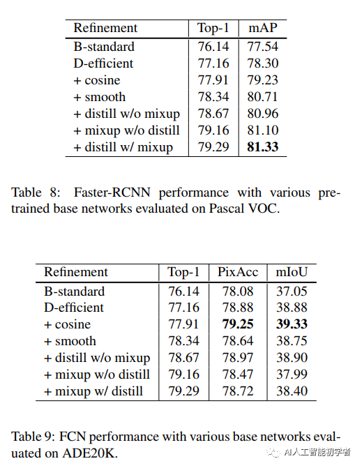
4.5,Experiment Results

5,Transfer Learning