catalogue
Introduction of linear regression model
Solution of regression coefficient
Linear regression in R language
Significance test of parameters -- t test
Verify various assumptions of the model
correlation analysis
- Draw a scatter chart and observe the correlation first
- Calculate according to the correlation coefficient, such as pearson correlation coefficient
- Absolute value of correlation
 0.8 is highly correlated, 0.5 to 0.8 is moderately correlated, 0.3-0.5 is weakly correlated, and less than 0.3 is almost irrelevant.
Regression analysis
- When the combination contains only one dependent variable and one independent variable, it is called simple linear regression model, on the contrary, it is multiple linear regression model.
Introduction of linear regression model

Solution of regression coefficient
- It is assumed that the mean value of the error term is 0 and the standard value is 0
 Normal distribution of
 - Construct likelihood function
- Take logarithm and sort it out
- Expand and derive
- Calculate partial regression coefficient
Linear regression in R language
lm(formula,data,subset,wrights,na.action)
#formula: specify the function, such as y~x1+x2, if y ~ Then it is related to all variables
#Subset sample subset
# weights
Significance test
#F test, anova function was used for analysis of variance
The theoretical value of F distribution under this degree of freedom can be obtained by using qf(0.95,5,34).
# modeling
model <- lm(Profit ~ ., data = train)
model

# Calculation of F statistics
result <- anova(model)
result

# Calculation of F statistics
RSS <- sum(result$`Sum Sq`[1:4])
df_RSS <- sum(result$Df[1:4])
ESS <- result$`Sum Sq`[5]
df_ESS <- sum(result$Df[5])
F <- (RSS/df_RSS)/(ESS/df_ESS)
F

qf(0.975,5,34)
Where RSS is the sum of squares of regression deviations (predicted value minus average value) and ESS is the sum of squares of errors (actual value minus predicted value)
Significance test of parameters -- t test
F test is used to test the model and t test is used to test a single parameter.
The value of the t-test can be obtained directly using the summary function
# Overview of the model
summary(model)

# Value of theoretical t distribution
n <- nrow(train)
p <- ncol(train)
t <- qt(0.975,n-p-1)
t
stepwise regression
- Forward regression: add variables step by step and adjust constantly
- Backward regression: stepwise deletion of variables
- Two way stepwise regression: deleted items can be added and added items can be deleted
Stepwise regression uses the step function
# Stepwise regression complete traversal selection
model2 <- step(model)
# Final model overview
summary(model2)
Verify various assumptions of the model
Multiple linearity test
Using the vif function of the car package
VIF is abbreviated as the expansion factor of variance. When 0 < VIF < 10, there is no multiple reproducibility. It exists from 10 to 100, and more than 100 is serious.
library(car)
vif(model2)
Normality test
#Draw histogram
hist(x = profit$Profit, freq = FALSE, main = 'Histogram of profit',
     ylab = 'Nuclear density value',xlab = NULL, col = 'steelblue')

#Add nuclear density map
lines(density(profit$Profit), col = 'red', lty = 1, lwd = 2)

#Add normal distribution map
x <- profit$Profit[order(profit$Profit)]
lines(x, dnorm(x, mean(x), sd(x)),
      col = 'black', lty = 2, lwd = 2.5)
Use PP chart or QQ chart
The abscissa of PP diagram is the cumulative probability, and the ordinate is the actual cumulative probability; The abscissa of QQ chart is the theoretical quantile and the ordinate is the actual quantile.
shapior test and k-s test
When the sample size is less than 5000, use shapiro test, otherwise use k-2 test.
If the P value is greater than the confidence level, the original hypothesis is accepted.
# Statistical method
shapiro.test(profit$Profit)
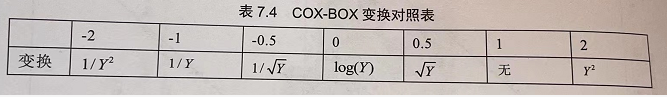
Mathematical transformation
When the variable does not obey the normal distribution, it carries out mathematical transformation, such as root opening, logarithm, and BOX-COX transformation.
# box-cox transformation
powerTransform(model2)
Independence test
Check whether the variables are independent.
# Independence test
durbinWatsonTest(model2)
Variance homogeneity test
The homogeneity of variance requires that the variance of the residual term of the model does not show a certain trend with the change of independent variables.
Whether there is a linear relationship is tested by BP, and the non-linearity is tested by White. If there is, the condition of homogeneity is not satisfied.
# Variance homogeneity test
ncvTest(model2)
model prediction
Using the predict function
# model prediction
pred <- predict(model2, newdata = test[,c('R.D.Spend','Marketing.Spend')])
ggplot(data = NULL, mapping = aes(pred, test$Profit)) +
  geom_point(color = 'red', shape = 19) +
  geom_abline(slope = 1, intercept = 0, size = 1) +
  labs(x = 'Estimate', y = 'actual value')