
Summary of face alignment and face key point detection based on Tensorflow framework with code (continuously updated)
Summary of face detection based on Tensorflow framework with code (continuously updated)
Summary of face matching based on Tensorflow framework with code (continuously updated)
recently used the open source face database WIDER FACE, 64_CASIA-FaceV5,CelebA,300W_LP and a private data set of nearly 200 photos made by itself reproduce the functions of face detection, face matching, face alignment, face key point detection, face attribute and living body detection, and integrate them into the wechat applet. All the above contents will be summarized by about 5 bloggers. All data set download links are attached below, and all complete codes are attached below GitHub link
Wide face dataset , including 32203 images and 393703 personal face images, which are different in scale, posture, occlusion, expression, dress, lighting, etc.
LFW dataset , is a commonly used test set for face recognition at present. The face images provided in it are all from natural scenes in life, so the recognition difficulty will increase. Especially, due to the influence of multi posture, illumination, expression, age, occlusion and other factors, even the photos of the same person are very different. And in some photos, more than one person's face may appear. For these multi face images, only the face in the central coordinate is selected as the target, and the faces in other areas are regarded as background interference. There are 13233 face images in LFW dataset, and each image gives the corresponding person's name. There are 5749 people in total, and most of them have only one picture. The size of each picture is 250X250, most of which are color images, but there are also a few black-and-white face images.
64_CASIA-FaceV5 The dataset contains 2500 Asian face images from 500 people.
CelebA 202599 face images with 10177 celebrity identities are included. Each image is marked with features, including face bbox annotation box, 5 face feature point coordinates and 40 attribute markers. It is widely used in face related computer vision training tasks, such as face attribute identification training, face detection training and landmark marking.
300W_LP The data set is a large pose 3D face alignment data set obtained by 3DDFA team based on the existing 2D face alignment data sets such as AFW, IBUG, HEPEP and FLWP, 3DMM annotation obtained by 3DMM fitting, changing posture, illumination and color, and flip (mirror) the original image.

1. Face alignment / key point business introduction
What is face alignment / face key detection
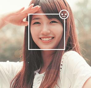
according to the input face image, automatically locate the key feature points of the face, such as the contour points of various parts of the face, such as eyes, tip of nose, corner of mouth, eyebrows and so on.
What is face alignment / face keys?
♦ 2D face find the coordinates of key points (x,y)
♦ 3D face uses deep learning to find facial feature contour information
♦ 5, 21, 29, 68, 96192... 1000, 8000 and other key points
■ applied to expression recognition, face editing, face makeup and 2D reconstruction
Evaluation index of face key point algorithm:
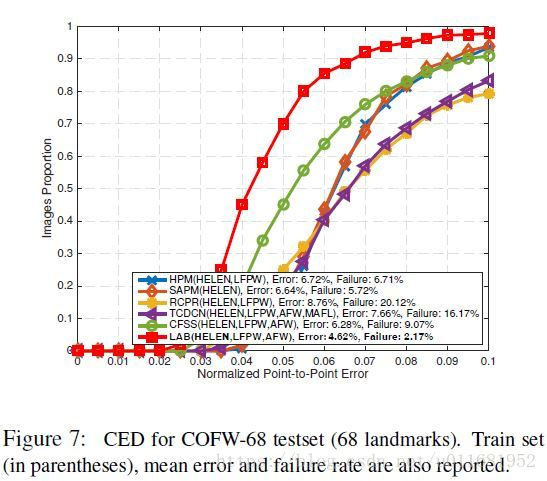
in the face key point location algorithm, the commonly used model evaluation index is the Cumulative Errors Distribution curve (CED): when the abscissa represents the Error between normalized points, the failure rate of LAB is 2.17%; In addition, Error in the figure refers to the average Error (MNE). Summary of common evaluation criteria for face alignment algorithms
 Reprint from above link
2. Introduction to face alignment / key point method
Traditional methods:
model based on shape learning: face model → point search → alignment → search and location of other points
ASM model is an active shape model, which abstracts the target object through the shape model. Its basic idea is as follows:
1. Firstly, the shape of the training samples is described by a set of face feature vectors to make the shape of the training samples as similar as possible;
2. Principal component analysis is used to statistically model the aligned shape vector;
3. The matching of specific objects is realized through the search of key points.
AAM model is an improvement on ASM model, using shape constraints and adding texture features of the whole face region. Like ASM, AAM is mainly divided into two stages: model establishment stage and model search and matching stage. The model establishment stage includes establishing shape model and texture model for training samples respectively, and then combining the two models to form AAM model.
Introduction to ASM and AAM algorithms
model based on cascade regression learning: initialization → calculation of features → calculation of transformation amount → update initialization
CPR: a cascade attitude regression algorithm is used to calculate the 2D attitude of the object in the image. The CPR algorithm gradually refines the randomly specified initial attitude, in which each attitude correction is determined by different regressors. Each regressor performs simple image measurement, which depends on the output of the previous regressor; The whole system automatically learns from the manually annotated training data set. CPR is not limited to rigid transformations: pose is any parametric change in the appearance of an object, such as deformability and the degrees of freedom of a joint object.
Deep learning methods:
Multilevel regression
DCNN: it belongs to the cascade regression core. The network has three levels of cascade neural network, which improves the problem of falling into local optimization caused by improper initial value. At the same time, with the help of CNN's high-quality feature extraction ability, it can obtain more accurate key point detection.
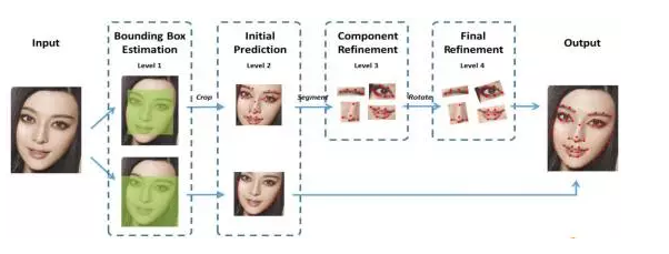
DCNN face + +: improved on the DCNN model, proposed a face key point detection algorithm from coarse to fine, and realized the high-precision location of 68 face key points. The algorithm divides the face key points into internal key points and contour key points. The internal key points include 51 key points including eyebrows, eyes, nose and mouth, and the contour key points include 17 key points. For internal and external key points, the algorithm uses two cascaded CNN for key point detection in parallel. The network structure is shown in the figure.
Multitasking
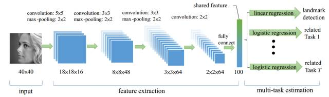
TCDCN: the original author believes that when carrying out the face key point detection task, combining some auxiliary information can help better locate the key points, such as gender, glasses, smile and face posture. The author combines the face key point detection (5 key points) with the four subtasks of gender, glasses, smile and face posture to form a multi task learning model. The model framework is shown in the figure below:
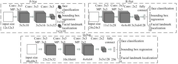
MTCNN: it contains three cascaded multi task convolutional neural networks, namely Proposal Network (P-Net), Refine Network (R-Net) and Output Network (O-Net). Each multi task convolutional neural network has three learning tasks, namely face classification, border regression and key point location. The network structure is shown in the figure:
Direct regression
vanella CNN: the network structure is the same as that of TCDCN, but its special feature is that it eliminates multi task learning and uses color images. Secondly, it replaces the loss function and uses the distance between two eyes for standardization. For details, please refer to: Facial feature point detection: VanillaCNN
Heat map
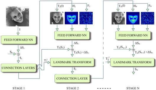
DAN: in 2017, the original author Kowalski et al. Proposed a new cascaded depth neural network - DAN (Deep Alignment Network). In the past, the input of cascaded neural network was a part of the image. Unlike in the past, the input of the network at each stage of DAN was the whole image. When the network uses the whole picture as the input, DAN can effectively overcome the problems caused by head posture and initialization, so as to get better detection effect. The reason why DAN can take the whole picture as input is that it adds Landmark Heatmaps. The use of key heatmaps is the main innovation of this paper. The basic framework of DAN is shown in the figure:
this blog is particularly meaningful. Thank the author don't know, don't learn, don't ask Deployment of deep learning network model -- face key point detection
2D face key point localization is in the development of → 3D face key point localization: firstly, 2D face key points are visible semantic information. At present, their detection accuracy is high, and 3D face key point detection is the focus of current research. Secondly, 3D face key point localization (dense face key point localization) mainly includes: Dense Face Alignment, DenseReg, FAN, 3DDFA, PRNet, etc
this project uses 300W-LP data set (see the beginning) to detect 68 key points of human face, and uses the data in AFW under landmarks in the file package, and its code is shown in the follow-up.
3. Face alignment / key point problems, challenges and Solutions
difficulties faced: solutions;
environmental change: data enhancement, illumination, rotation;
pose change: pose classification and face alignment;
expression change: data enhancement, GAN;
occlusion problem: 3D face key point location;


4.Tensorflow + SENet implementation and model optimization
overall analysis: data → network structure → 68 point 136 dimensional vector
introduction to SENet model: squeeze and exception networks (SENet) is a new image recognition structure released by automatic driving company Momenta in 2017. It improves the accuracy by modeling the correlation between feature channels and strengthening important features.
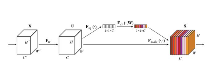
the above figure is the Block unit of SENet. Ftr in the figure is the traditional convolution structure, and X and U are the input (c'xH'xW ') and output (CxHxW) of Ftr, which have existed in the previous structure. The added part of SENet is the structure after U: first make a Global Average Pooling for U (Fsq(.) in the figure), The author calls it the Squeeze process), and the output 1x1xC data goes through two-stage full connection (Fex(.) in the figure), The author calls it the exception process), and finally limits it to the range of [0,1] with sigmoid (self gating mechanism in the paper), and multiplies this value as a scale to the C channels of U as the input data of the next level. The principle of this structure is to enhance the important features and weaken the unimportant features by controlling the size of scale, so as to make the extracted features more directional
face key point positioning data preparation
read the image data, and the key codes are as follows:
m = loadmat("300w-lp-dataset/300W_LP/landmarks/AFW/AFW_134212_1_0_pts.mat")

landmark = m['pts_2d']

m_data = cv2.imread("300w-lp-dataset/300W_LP/AFW/AFW_134212_1_0.jpg")

for i in range(68):
    cv2.circle(m_data, (int(landmark[i][0]), int(landmark[i][1])),
                        2, (0,255, 0), 2)
cv2.imshow("11", m_data)
cv2.waitKey(0)
an example of reading an image is as follows:
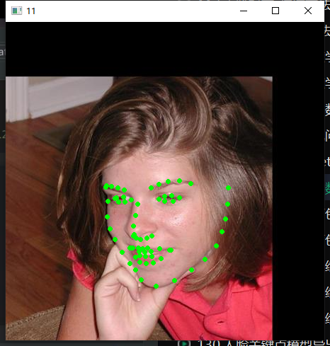
after reading the image data, the following key codes for writing data are:
landmark_path_data = "300w-lp-dataset/300W_LP/landmarks"
landmark_path_folders = glob.glob(landmark_path_data + "/*")
#The obtained files are stored in the list
landmark_anno_list = []
#Traverse all subfolders under the landmarks folder
for f in landmark_path_folders:
    landmark_anno_list += glob.glob(f + "/*.mat")
print(landmark_anno_list)

#Save model
writer_train = tf.python_io.TFRecordWriter("train.tfrecords")
writer_test = tf.python_io.TFRecordWriter("test.tfrecords")
#Traverse all files in the list
for idx in range(landmark_anno_list.__len__()):
    landmark_info = landmark_anno_list[idx]
    im_path = landmark_info.replace("300W_LP/landmarks","300W_LP").replace("_pts.mat", ".jpg")
    print(im_path)
    im_data = cv2.imread(im_path)
    #Take image
    landmark = loadmat(landmark_info)['pts_2d']
    #Get face keys

    x_max = int(np.max(landmark[0:68, 0]))
    x_min = int(np.min(landmark[0:68, 0]))

    y_max = int(np.max(landmark[0:68, 1]))
    y_min = int(np.min(landmark[0:68, 1]))
    #Adjust the position of face frame
    y_min = int(y_min - (y_max - y_min) * 0.3)
    y_max = int(y_max + (y_max - y_min) * 0.05)

    x_min = int(x_min - (x_max - x_min) * 0.05)
    x_max = int(x_max + (x_max - x_min) * 0.05)

    face_data = im_data[y_min : y_max, x_min : x_max]
    sp = face_data.shape
    im_point = []
    for p in range(68):
        im_point.append((landmark[p][0] - x_min) * 1.0 / sp[1])
        im_point.append((landmark[p][1] - y_min) * 1.0 / sp[0])

    face_data = cv2.resize(face_data, (128, 128))
    ex = tf.train.Example(
        features = tf.train.Features(
            feature = {
                "image" : tf.train.Feature(
                    bytes_list = tf.train.BytesList(value = [face_data.tobytes()])
                ),
                "label": tf.train.Feature(
                    float_list=tf.train.FloatList(value=im_point)
                )
            }
        )
    )
    if idx > landmark_anno_list.__len__() * 0.9:
        writer_test.write(ex.SerializeToString())
    else:
        writer_train.write(ex.SerializeToString())

writer_test.close()
writer_train.close()
Training, debugging and testing of face key point location model
after the data is packaged, the next step is to train the face key point location model, and the key codes are as follows:
# read data
def get_one_batch(batch_size, type):
    if type == 0:       #train
        file_list = tf.gfile.Glob("train*.tfrecords")
    else:
        file_list = tf.gfile.Glob("test*.tfrecords")
    reader = tf.TFRecordReader()
    filename_queue = tf.train.string_input_producer(
        file_list, num_epochs = None, shuffle = True
    )
    _,se = reader.read(filename_queue)
    if type == 0:
        batch = tf.train.shuffle_batch([se], batch_size,
                                       capacity = batch_size,
                                       min_after_dequeue = batch_size // 2)
    else:
        batch = tf.train.batch([se], batch_size,
                               capacity = batch_size)
    features = tf.parse_example(batch, features = {
        'image':tf.FixedLenFeature([], tf.string),
        'label':tf.FixedLenFeature([136], tf.float32)
    })
    batch_im = features['image']
    batch_label = features['label']
    batch_im = tf.decode_raw(batch_im, tf.uint8)
    batch_im= tf.cast(tf.reshape(batch_im,
                                 (batch_size, 128, 128, 3)), tf.float32)
    return batch_im, batch_label

#net
input_x = tf.placeholder(tf.float32, shape = [None, 128, 128, 3])
label = tf.placeholder(tf.float32, shape=[None, 136])

logits = SENet(input_x, is_training = True, keep_prob = 0.8)
#loss
loss = tf.losses.mean_squared_error(label, logits)
reg_set = tf.get_collection(tf.GraphKeys.REGULARIZATION_LOSSES)
l2_loss = tf.add_n(reg_set)

#learn
global_step = tf.Variable(0, trainable=False)
lr = tf.train.exponential_decay(0.001, global_step,
                                decay_steps = 1000,
                                decay_rate = 0.98,
                                staircase = True)
update_ops = tf.get_collection(tf.GraphKeys.UPDATE_OPS)
with tf.control_dependencies(update_ops):
    train_op = tf.train.AdamOptimizer(lr).minimize(l2_loss + loss, global_step)
#save
saver = tf.train.Saver(tf.global_variables())

tr_im_batch, tr_label_batch = get_one_batch(32, 0)
te_im_batch, te_label_batch = get_one_batch(32, 1)
after the model enters training, use tensorboard to observe the change trend of loss function value, as shown in the following figure:

after the training, the key codes of exporting the model pb file (model solidification) are as follows:
#net
input_x = tf.placeholder(tf.float32, shape = [1, 128, 128, 3])

logits = SENet(input_x, is_training = False, keep_prob = 1.0)
print(logits)
saver = tf.train.Saver(tf.global_variables())
#session
with tf.Session() as session:
    coord = tf.train.Coordinator()
    tf.train.start_queue_runners(sess = session, coord = coord)

    init_op = tf.group(tf.global_variables_initializer(), tf.local_variables_initializer())
    session.run(init_op)

    ckpt = tf.train.get_checkpoint_state("models")
    saver.restore(session, ckpt.model_checkpoint_path)
    output_graph_def = tf.graph_util.convert_variables_to_constants(session,
                                                                    session.graph.as_graph_def(),
                                                                    ['fully_connected_9/Relu'])
    with tf.gfile.FastGFile("landmark.pb", "wb") as f:
        f.write(output_graph_def.SerializeToString())
        f.close()
after saving the pb file, the model is tested. The key code of human face key point model test is as follows:
pb_path = "landmark.pb"
sess = tf.Session()
with sess.as_default():
    with tf.gfile.FastGFile(pb_path, "rb") as f:
        graph_def = sess.graph_def
        graph_def.ParseFromString(f.read())
        tf.import_graph_def(graph_def, name = "")

im_list = glob.glob("images/*")

landmark = sess.graph.get_tensor_by_name("fully_connected_9/Relu:0")

for im_url in im_list:
    print(im_url)
    im_data = cv2.imread(im_url)
    im_data = cv2.resize(im_data, (128,128))

    pred = sess.run(landmark, {"Placeholder:0" : np.expand_dims(im_data, 0)})
    print(pred)
    pred = pred[0]
    for i in range(0, 136, 2):
        cv2.circle(im_data, (int(pred[i] * 128), int(pred[i+1] * 128)),
                   2, (0, 255, 0), 2)
    cv2.imshow("11",im_data)
    cv2.waitKey(0)
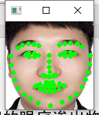
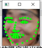
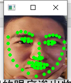
test on the personal data set to observe whether the detection of face key point location is accurate (according to the result diagram, the effect of face key point location in the personal data set can be further improved. Next, integrate multiple training sets for training, and expand the private data set for multiple tests to find the optimal model)
Optimization and improvement strategy of face key point location model
- Other backbone networks are selected for experiments, such as other edge detection models, etc;
- Select composite loss function or more suitable optimizer;
- Enhance data processing. Or use GAN network;
- A module for attitude classification can be added to solve the problem of key point detection affected by multiple attitudes.