1, Introduction
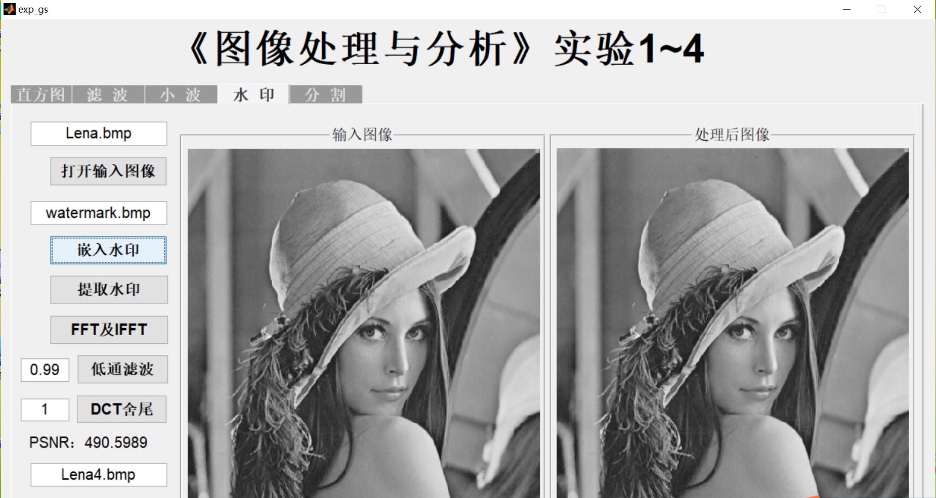
GUI image histogram, filtering, wavelet transform and segmentation processing system based on MATLAB
Part1 introduction to the wavelet transform
1,Origin of the wavelet transform:
The theories of Wavelet originate from diffierent areas of study:
-
Engineering
-
Time-frequency analysis and Multiresolution Analysis
-
Computer Vision
-
Pyramidal algorithm
-
Physics
-
Pure Mathematics
2. Multiresolution Analysis (MRA - Multiresolution Analysis and processing)
-
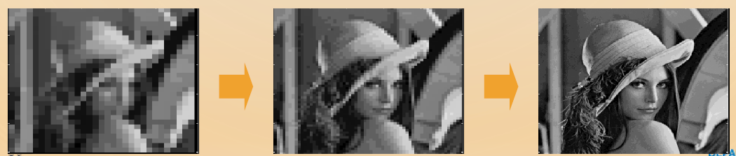
Multiresolution analysis is about analyzing a signal based on the information appeared in different scales of such signal – to mimic human beings in analyzing signals.
-
A signal of a certain "scale" refers to its best approximation at a certain resolution
-
By "traveling" from the coarse scales toward the fine scales, one zooms in and arrives at a more exact representation of the given signal
3. The discrete wavelet transform
A simple way to implement MAR is by using the Discrete Wavelet Transform(DWT):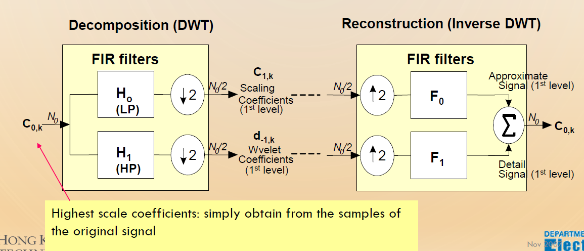
The definition of wavelet transform shows that the wavelet analysis is a measure of similarity the basis functions(wavelets) and the original function .The coefficients ,named H0 for Low Pass Filter, and H1 for High Pass Filter, caculated indicate how close the function is to the danghter wavelet at that particular scale.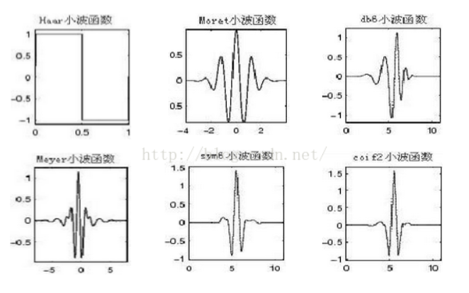
Part2 decomposition (DWT) and reconstruction (inverse DWT) – discrete wavelet decomposition and reconstruction
For discrete wavelet transform, because many wavelet functions are not orthogonal functions, one Scaling Coefficients and one Wavelet Coefficients are needed Therefore, the original signal function can be decomposed into a linear combination of scale function (coefficient) and wavelet function (coefficient). In this function, scale function generates low-frequency part and wavelet function generates high-frequency part.
1. One dimensional Haar wavelet transform decomposition
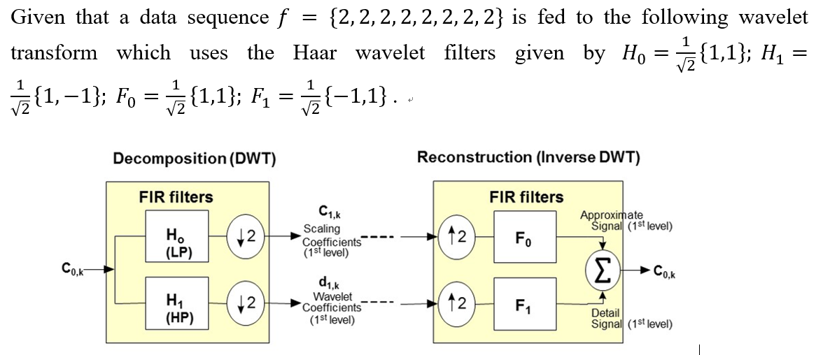
When the discrete signal passes through Haar wavelet transform, firstly, the information carried by the signal will be compressed to obtain N/2 data points for storage. Then these point information is characterized by these Scaling Coefficients. For discrete signals, they may have high-frequency and low-frequency components, while wavelet coefficients or detail coefficients represent its high-frequency part.
Down sampling in wavelet is to sample the signal every other point in order to compress and store the information.
Upsampling in wavelet is to insert zeros every other point in order to reconstruct the signal.
The filtering process of the signal is mathematically equivalent to the convolution of the signal and the impulse response of the filter.
Decomposition LP filter (discrete convolution operator):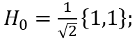
Decomposition HP filter (discrete convolution operator):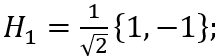
Discrete time convolution theorem:
"Discrete convolution" is a special operation in which two discrete sequences x(n) and h(n) are multiplied and added according to certain rules. The specific formula can be expressed as: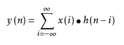
Where y (n) is a new sequence obtained after convolution operation.
Discrete convolution is widely used in engineering. For example, in the field of digital image processing, in order to filter the digital signal, the image signal C(n) expressed as a discrete sequence can be discretely convoluted with the impulse response h(n) of the digital filter.
Wavelet function of multiresolution analysis Ψ (t) Scaling function φ (t) Satisfy the two-scale difference equation: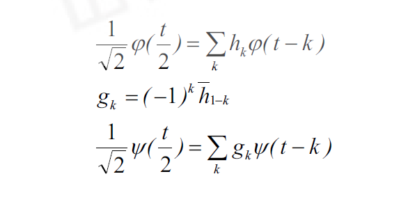
Each layer of multi-resolution analysis decomposes the signal f(t) into low-frequency part and high-frequency part through a low-pass filter and band-pass filter. The characteristics of low-pass filter are determined by wavelet function Ψ (x) It is determined that the characteristics of the band-pass filter are determined by the scale function φ (x) OK. The decomposed coefficient consists of two parts: low-frequency coefficient vector c1 and high-frequency coefficient vector d1. The low-frequency coefficient vector c1 is obtained by convolution of the impulse response of the signal and the low-pass filter (determined by the wavelet function), and the high-frequency coefficient vector d1 is obtained by convolution of the signal and the band-pass filter (determined by the scale function).
2. One dimensional Haar wavelet transform reconstruction
Inverse transformation process:
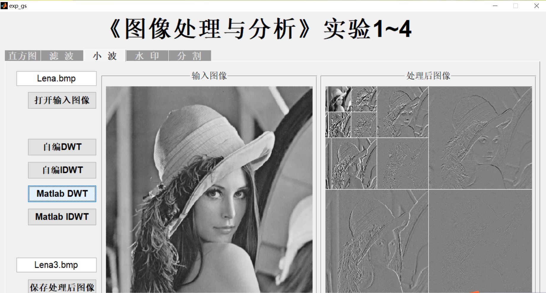
3. Two dimensional Haar wavelet transform
Two dimensional image signal
For two-dimensional image signals, two-dimensional wavelet multi-resolution decomposition can be realized by filtering in the horizontal and vertical directions respectively. Figure 2.5 shows the division of sub images after decomposition by two-dimensional discrete wavelet transform. Of which:
(l)LL subband is a wavelet coefficient generated by convolution of two directions using low-pass wavelet filter. It is an approximate representation of the image.
(2)HL subband is a wavelet coefficient generated by convolution in the row direction with low-pass wavelet filter and then convolution in the column direction with high-pass wavelet filter. It represents the horizontal singularity of the image. (horizontal subband)
(3)LH subband is a wavelet coefficient generated by convolution in the row direction with high-pass wavelet filter and then convolution in the column direction with low-pass wavelet filter. It represents the vertical singularity of the image. (vertical subband)
(4)HH subband is a wavelet coefficient generated by convolution of two directions using high pass wavelet filter, which represents the diagonal edge characteristics of the image. (diagonal subband)
The first letter indicates the processing of column direction and the second letter indicates the processing of row direction. The singular characteristics of the image are retained when passing through low pass and filtered when passing through high pass.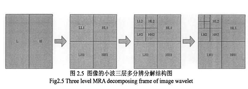
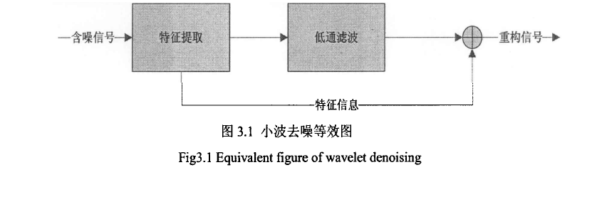
Wavelet denoising method is to find the best image from the actual signal space to the wavelet function space, so as to obtain the best recovery of the original signal.
At present, wavelet denoising methods can be divided into three categories:
The first kind of method - wavelet transform modulus maximum denoising method
The principle of wavelet transform modulus maximum is used to denoise. It is based on simultaneous interpreting of the different propagation characteristics of signals and noises in different scales of wavelet transform, eliminating the modulus maxima generated by noise, preserving the modulus maximum value corresponding to the signal, and then reconstructing the wavelet coefficients by using the maximum modulus of the modulus, and then recovering the signal.
The second kind of method - wavelet coefficient correlation denoising method
After the wavelet transform of the noisy signal, the correlation of wavelet coefficients between adjacent scales is calculated, and the types of wavelet coefficients are distinguished according to the correlation, so as to make a choice, and then the signal is reconstructed directly;
The third kind of method - wavelet transform threshold de creation method
Wavelet threshold denoising method, which considers that the wavelet coefficients corresponding to the signal contain important information of the signal, with large amplitude but small number, while the wavelet coefficients corresponding to the noise are uniformly distributed, with large number but small amplitude.
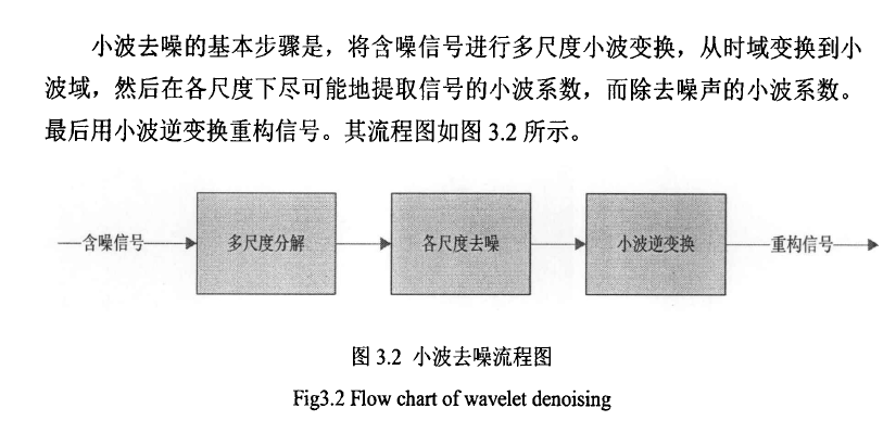
4. Wavelet threshold shrinkage denoising method:
1. Basic idea of wavelet threshold denoising:
The basic idea of wavelet threshold denoising proposed by Donoho is that after the signal is transformed by wavelet (Mallat algorithm is adopted), the wavelet coefficient generated by the signal contains important information of the signal. After the signal is decomposed by wavelet, the wavelet coefficient is larger, the wavelet coefficient of noise is smaller, and the wavelet coefficient of noise is smaller than the wavelet coefficient of signal. By selecting an appropriate threshold, Wavelet coefficients greater than the threshold are considered to be generated by signals and should be retained. Those less than the threshold are considered to be generated by noise and set to zero to achieve the purpose of denoising. The basic steps are:
(1) Decomposition: select a wavelet with N layers to decompose the signal;
(2) Threshold processing process: after decomposition, select an appropriate threshold and quantify the coefficients of each layer with the threshold function;
(3) Reconstruction: reconstruct the signal with the processed coefficients.
2. Basic problems of wavelet threshold denoising
The basic problem of wavelet threshold denoising includes three aspects: the selection of wavelet basis, the selection of threshold and the selection of threshold function.
(1) Selection of wavelet base: generally, we hope that the selected wavelet meets the following conditions: orthogonality, high vanishing moment, compact support, symmetry or antisymmetry. But in fact, wavelets with the above properties cannot exist, because wavelets are symmetric or antisymmetric, only Haar wavelets, and high vanishing moment and compactly supported are a pair of contradictions. Therefore, in application, wavelets with compactly supported are generally selected, and more appropriate wavelets are selected according to the characteristics of signals.
(2) Selection of threshold: an important factor that directly affects the denoising effect is the selection of threshold. Different threshold selection will have different denoising effects. At present, there are mainly general threshold (VisuShrink), surelink threshold, Minimax threshold, Bayes shrink threshold, etc.
(3) Selection of threshold function: threshold function is the rule to modify wavelet coefficients. Different functions reflect different strategies to deal with wavelet coefficients. There are two most commonly used threshold functions: one is hard threshold function, and the other is soft threshold function. There is also a Garrote function between soft and hard threshold functions.
In addition, for the evaluation of denoising effect, the signal-to-noise ratio (SNR) of the signal and the root mean square error (MSE) between the estimated signal and the original signal are often used to judge.
2, Source code
unction varargout = exp_gs(varargin)
% EXP_GS M-file for exp_gs.fig
% EXP_GS, by itself, creates a new EXP_GS or raises the existing
% singleton*.
%
% H = EXP_GS returns the handle to a new EXP_GS or the handle to
% the existing singleton*.
%
% EXP_GS('CALLBACK',hObject,eventData,handles,...) calls the local
% function named CALLBACK in EXP_GS.M with the given input arguments.
%
% EXP_GS('Property','Value',...) creates a new EXP_GS or raises the
% existing singleton*. Starting from the left, property value pairs are
% applied to the GUI before exp_gs_OpeningFcn gets called. An
% unrecognized property name or invalid value makes property application
% stop. All inputs are passed to exp_gs_OpeningFcn via varargin.
%
% *See GUI Options on GUIDE's Tools menu. Choose "GUI allows only one
% instance to run (singleton)".
%
% See also: GUIDE, GUIDATA, GUIHANDLES
% Edit the above text to modify the response to help exp_gs
% Last Modified by GUIDE v2.5 30-Jun-2010 13:33:39
% Begin initialization code - DO NOT EDIT
gui_Singleton = 1;
gui_State = struct('gui_Name', mfilename, ...
'gui_Singleton', gui_Singleton, ...
'gui_OpeningFcn', @exp_gs_OpeningFcn, ...
'gui_OutputFcn', @exp_gs_OutputFcn, ...
'gui_LayoutFcn', [] , ...
'gui_Callback', []);
if nargin && ischar(varargin{1})
gui_State.gui_Callback = str2func(varargin{1});
end
if nargout
[varargout{1:nargout}] = gui_mainfcn(gui_State, varargin{:});
else
gui_mainfcn(gui_State, varargin{:});
end
% End initialization code - DO NOT EDIT
% --- Executes just before exp_gs is made visible.
function exp_gs_OpeningFcn(hObject, eventdata, handles, varargin)
% This function has no output args, see OutputFcn.
% hObject handle to figure
% eventdata reserved - to be defined in a future version of MATLAB
% handles structure with handles and user data (see GUIDATA)
% varargin command line arguments to exp_gs (see VARARGIN)
% Choose default command line output for exp_gs
handles.output = hObject;
% Update handles structure
guidata(hObject, handles);
% UIWAIT makes exp_gs wait for user response (see UIRESUME)
% uiwait(handles.figure1);
% --- Outputs from this function are returned to the command line.
function varargout = exp_gs_OutputFcn(hObject, eventdata, handles)
% varargout cell array for returning output args (see VARARGOUT);
% hObject handle to figure
% eventdata reserved - to be defined in a future version of MATLAB
% handles structure with handles and user data (see GUIDATA)
% Get default command line output from handles structure
varargout{1} = handles.output;
function edit1_Callback(hObject, eventdata, handles)
% hObject handle to edit1 (see GCBO)
% eventdata reserved - to be defined in a future version of MATLAB
% handles structure with handles and user data (see GUIDATA)
% Hints: get(hObject,'String') returns contents of edit1 as text
% str2double(get(hObject,'String')) returns contents of edit1 as a double
% --- Executes during object creation, after setting all properties.
function edit1_CreateFcn(hObject, eventdata, handles)
% hObject handle to edit1 (see GCBO)
% eventdata reserved - to be defined in a future version of MATLAB
% handles empty - handles not created until after all CreateFcns called
% Hint: edit controls usually have a white background on Windows.
% See ISPC and COMPUTER.
if ispc && isequal(get(hObject,'BackgroundColor'), get(0,'defaultUicontrolBackgroundColor'))
set(hObject,'BackgroundColor','white');
end
% --- Executes on button press in pushbutton1.
function pushbutton1_Callback(hObject, eventdata, handles)
% hObject handle to pushbutton1 (see GCBO)
% eventdata reserved - to be defined in a future version of MATLAB
% handles structure with handles and user data (see GUIDATA)
ImgPath=get(handles.edit1,'String');
global img_1;
img_1=imread(ImgPath);
axes(handles.axes1);
imshow(img_1);
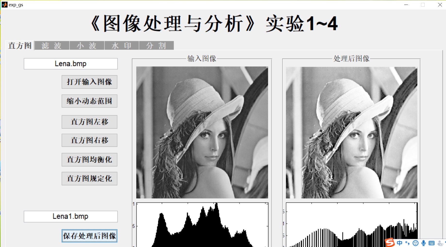
global histogram1;
histogram1=zeros(1,256);
[sizex,sizey]=size(img_1);
for ii=1:sizex % Calculate histogram
for jj=1:sizey
histogram1(img_1(ii,jj)+1)=histogram1(img_1(ii,jj)+1)+1;
end
end
maxhisto1=sum(histogram1);% normalization
histogram1=histogram1/maxhisto1;
axes(handles.axes2);
bar(0:255,histogram1);
axis([0 255 0 max(histogram1)]);
% --- Executes on button press in pushbutton2.
function pushbutton2_Callback(hObject, eventdata, handles)
% hObject handle to pushbutton2 (see GCBO)
% eventdata reserved - to be defined in a future version of MATLAB
% handles structure with handles and user data (see GUIDATA)
global img_1;
[sizex,sizey]=size(img_1);
for ii=1:sizex % Reduce dynamic range
for jj=1:sizey
img_1tmp(ii,jj)=floor(img_1(ii,jj)/2)+64;
end
end
global img_11;
img_11=img_1tmp;
axes(handles.axes3);
imshow(img_11);
histogram2=zeros(1,256);
for ii=1:sizex
for jj=1:sizey
histogram2(img_11(ii,jj)+1)=histogram2(img_11(ii,jj)+1)+1;
end
end
maxhisto2=sum(histogram2);
histogram2=histogram2/maxhisto2;
axes(handles.axes4);
bar(0:255,histogram2);
axis([0 255 0 max(histogram2)]);
% --- Executes on button press in pushbutton3.
function pushbutton3_Callback(hObject, eventdata, handles)
% hObject handle to pushbutton3 (see GCBO)
% eventdata reserved - to be defined in a future version of MATLAB
% handles structure with handles and user data (see GUIDATA)
global img_1;
[sizex,sizey]=size(img_1);
for ii=1:sizex % Histogram shift left
for jj=1:sizey
img_1tmp(ii,jj)=img_1(ii,jj)-30;
end
end
global img_11;
img_11=img_1tmp;
axes(handles.axes3);
imshow(img_11);
histogram3=zeros(1,256);
for ii=1:sizex
for jj=1:sizey
histogram3(img_11(ii,jj)+1)=histogram3(img_11(ii,jj)+1)+1;
end
end
maxhisto3=sum(histogram3);
histogram3=histogram3/maxhisto3;
axes(handles.axes4);
bar(0:255,histogram3);
axis([0 255 0 max(histogram3)]);
% --- Executes on button press in pushbutton4.
function pushbutton4_Callback(hObject, eventdata, handles)
% hObject handle to pushbutton4 (see GCBO)
% eventdata reserved - to be defined in a future version of MATLAB
% handles structure with handles and user data (see GUIDATA)
global img_1;
[sizex,sizey]=size(img_1);
for ii=1:sizex % Histogram shift right
for jj=1:sizey
img_1tmp(ii,jj)=img_1(ii,jj)+30;
end
end
global img_11;
img_11=img_1tmp;
axes(handles.axes3);
imshow(img_11);
histogram4=zeros(1,256);
for ii=1:sizex
for jj=1:sizey
histogram4(img_11(ii,jj)+1)=histogram4(img_11(ii,jj)+1)+1;
end
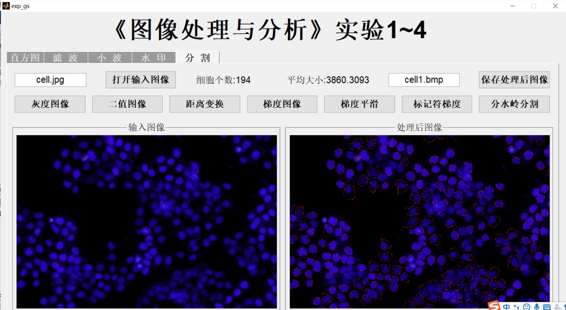
end3, Operation results
4, Remarks
Complete code or write on behalf of QQ1575304183