Welcome to more highlights
Pay attention to me, learn common algorithms and data structures, solve multiple problems and reduce dimension.
The algorithm implemented in this paper comes from the following paper
References: Bilateral Normal Filtering for Mesh Denoising, https://ieeexplore.ieee.org/document/5674028
Algorithm principle and process
Algorithm principle
Firstly, bilateral filtering is used to adjust the normal direction of the face, and then the vertex is adjusted according to the normal direction, so that the normal direction of the face is as close as possible to the adjusted normal direction.
Normal adjustment
n k + 1 ( f i ) = 1 K p ∑ j ∈ Ω ( i ) A j W s ( ∣ ∣ c i − c j ∣ ∣ ) W r ( ∣ ∣ n k ( f i ) − n k ( f j ) ∣ ∣ ) ⋅ n k ( f j ) n^{k+1}(f_i) = \frac{1}{K_p} \displaystyle \sum_{j\in Ω(i)}A_{j}W_s(||c_i-c_j||)W_r(||n^k(f_i)-n^k(f_j)||)\cdot n^k(f_j) nk+1(fi)=Kp1j∈Ω(i)∑AjWs(∣∣ci−cj∣∣)Wr(∣∣nk(fi)−nk(fj)∣∣)⋅nk(fj)
In the above formula
k represents the number of iterations
n k ( f i ) surface show through too k second Overlap generation after The first i individual noodles of method towards n^k(f_i) represents the normal direction of the ith face after K iterations nk(fi) represents the normal direction of the ith face after k iterations
c i generation surface The first i individual noodles of in heart c_i represents the center of the ith face ci represents the center of the ith face
Ω ( i ) surface show The first i individual noodles of place have adjacent noodles Ω (i) represents all adjacent faces of the ith face Ω (i) represents all adjacent faces of the ith face
A j surface show The first j individual noodles of noodles product A_j represents the area of the j-th face Aj , represents the area of the j-th face
W s ( x ) yes one individual high Si letter number = e − x 2 2 σ s 2 , his in x = c i − c j of long degree , σ s yes can transfer ginseng number , book second real present in take value by place have adjacent noodles in heart difference value of flat all value W_s(x) is a Gaussian function = e^{-\frac{x^2}{2\sigma^2_s}}, \ \ where x = C_ i-c_ Length of J, \ sigma_s is an adjustable parameter, \ \ the value in this implementation is the average value of the center difference of all adjacent planes Ws (x) is a Gaussian function = e − 2 σ s2 − x2, where x = the length of CI − cj, σ s , is an adjustable parameter. In this implementation, the value is the average value of the center difference of all adjacent planes
W r ( x ) yes one individual high Si letter number = e − x 2 2 σ r 2 , his in x = n k ( f i ) − n k ( f j ) of long degree , σ r yes can transfer ginseng number , book second real present in take value by 1 W_r(x) is a Gaussian function = e^{-\frac{x^2}{2\sigma^2_r}, \ \ where x = the length of n ^ k (f_i) - n ^ k (f_j), \ sigma_r is an adjustable parameter, \ \ the value in this implementation is 1 Wr (x) is a Gaussian function = e − 2 σ r2 − x2, where x = the length of NK (FI) − nk(fj), σ r , is an adjustable parameter, and the value in this implementation is 1
K p = ∑ j ∈ Ω ( i ) A j W s ( ∣ ∣ c i − c j ∣ ∣ ) W r ( ∣ ∣ n k ( f i ) − n k ( f j ) ∣ ∣ ) K_p = \displaystyle \sum_{j\in Ω(i)}A_{j}W_s(||c_i-c_j||)W_r(||n^k(f_i)-n^k(f_j)||) Kp=j∈Ω(i)∑AjWs(∣∣ci−cj∣∣)Wr(∣∣nk(fi)−nk(fj)∣∣)
The normal adjustment can be used many times, and the specific parameters can be adjusted k.
After each calculation, the normal direction shall be normalized.
Point top recovery
It is very difficult to calculate all vertices according to the normal direction. Here, a one-step Gaussian iteration method is adopted, and only one point top is adjusted at a time, so that the normal direction is as close to the calculated normal direction as possible.
According to the definition, we have the following formula
{ n f ⋅ ( x j − x i ) = 0 n f ⋅ ( x k − x j ) = 0 n f ⋅ ( x i − x k ) = 0 \left\{\begin{array}{l}n_f\cdot (x_j-x_i)=0\\n_f\cdot (x_k-x_j)=0\\n_f\cdot (x_i-x_k)=0\end{array}\right. ⎩⎨⎧nf⋅(xj−xi)=0nf⋅(xk−xj)=0nf⋅(xi−xk)=0
x i , x j , x k yes some individual noodles of three spot , n f yes transfer whole after of method towards , upper State common type surface show each strip edge all want Hang straight to method Line x_i, x_j, x_k is the three points of a face, n_f is the adjusted normal direction. The above formula means that each edge should be perpendicular to the normal xi, xj, xk , are the three points of a face, and nf , is the adjusted normal direction. The above formula indicates that each edge should be perpendicular to the normal
I Men of order mark yes send upper State common type More meet near to 0 More good Our goal is to make the above formula as close to 0 as possible Our goal is to make the above formula as close to 0 as possible
You can get an energy equation
E = ∑ f k ∑ i , j ∈ f k ( n k ⋅ ( x j − x i ) ) 2 E=\displaystyle \sum_{f_k}\displaystyle \sum_{i,j \in f_k}(n_k\cdot (x_j-x_i))^2 E=fk∑i,j∈fk∑(nk⋅(xj−xi))2
Now all we have to do is find a set of vertices to minimize E.
Here, only one point is moved at a time to minimize E.
By deriving the above equation and making it equal to 0, the calculation formula of a certain point can be deduced
x i n e w = x i + 1 N i ∑ f j ∈ Ω ( i ) n j ⋅ ( n j ⋅ ( c j − x i ) ) x^{new}_i=x_i+\frac {1}{N_i} \displaystyle \sum_{f_j \in Ω(i)}n_j \cdot (n_j \cdot (c_j-x_i)) xinew=xi+Ni1fj∈Ω(i)∑nj⋅(nj⋅(cj−xi))
N i surface show top spot of degree N_i represents the degree of the vertex Ni represents the degree of the vertex
Ω ( i ) yes The first i individual spot place have adjacent noodles Ω (i) is all adjacent surfaces of the ith point Ω (i) is all adjacent surfaces of the ith point
x i yes primary come want change turn of spot x_i is the original point to be changed The original point of change is xi
c j yes his he top spot of sit mark c_j is the coordinates of the other vertices cj is the coordinate of other vertices
n j yes The first j individual noodles of order mark method towards n_j is the target normal direction of the j-th plane nj , is the target normal direction of the j-th plane
In the above process, all vertices can be restored each time, and the parameters can be adjusted for many times. This implementation adopts 8 times.
Algorithm implementation
Code github https://github.com/LightningBilly/ACMAlgorithms/tree/master/%E5%9B%BE%E5%BD%A2%E5%AD%A6%E7%AE%97%E6%B3%95/%E4%B8%89%E8%A7%92%E7%BD%91%E6%A0%BC%E7%AE%97%E6%B3%95/MeshWork/src/hw3
#include <iostream>
#include <fstream>
#include <sstream>
#include "../../PolyMesh/IOManager.h"
#include <string>
#include <unistd.h>

using namespace std;
using namespace acamcad;
using namespace polymesh;

void hw3()
{
    puts("hw3");

    char buffer[500];
    getcwd(buffer, 500);
    printf("The current directory is: %s/../\n", buffer);
    string mesh_path = buffer;
    mesh_path += "/../src/hw3/bunny_random.obj";
    double SigmaCenter, SigmaNormal=1;
    double NormalIterNum=8, VertexIterNum=8;

    PolyMesh* mesh = new PolyMesh();
    loadMesh(mesh_path, mesh);

    mesh->updateMeshNormal();
    std::vector<MVector3> NewNormal(mesh->numPolygons());
    std::vector<double> FaceArea(mesh->numPolygons());
    std::vector<MPoint3> FaceCenter(mesh->numPolygons());

    for (MPolyFace* fh : mesh->polyfaces())
    {
        int f_id = (*fh).index();
        NewNormal[f_id] = (*fh).normal();
        std::vector<MVert*> P;
        for (FaceVertexIter vv_it = mesh->fv_iter(fh); vv_it.isValid(); ++vv_it)
        {
            P.push_back(*vv_it);
        }
        auto e12 = P[1]->position() - P[0]->position();
        auto e13 = P[2]->position() - P[0]->position();
        double area = cross(e12, e13).norm() * 0.5;
        FaceArea[f_id] = area;
        FaceCenter[f_id] = mesh->calculatFaceCenter(fh);
    }

    /*
     * Standard deviation parameters of calculation points
     * Make a difference between the midpoint of all adjacent surfaces
     * Finally divided by three times the face
     */
    SigmaCenter = 0;
    for (MPolyFace* fh : mesh->polyfaces())
    {
        int f_id = (*fh).index();
        for (FaceFaceIter nei_fh = mesh->ff_iter(fh); nei_fh.isValid(); ++nei_fh)
        {
            int ff_id = (*nei_fh)->index();
            SigmaCenter += (FaceCenter[f_id] - FaceCenter[ff_id]).norm();
        }
    }
    SigmaCenter /= mesh->numPolygons() * 3;

    /*
     * The normal direction is calculated by using the normal iterative formula
     */
    for (int i = 0; i < NormalIterNum; i++)
    {
        for (MPolyFace* fh : mesh->polyfaces())
        {
            double Kp = 0;
            MVector3 NewN(0, 0, 0);
            int fh_id = (*fh).index();
            for (FaceFaceIter nei_fh = mesh->ff_iter(fh); nei_fh.isValid(); ++nei_fh)
            {
                int nei_fh_id = (*nei_fh)->index();
                double delta_center = (FaceCenter[fh_id] - FaceCenter[nei_fh_id]).norm();
                double delta_normal = (NewNormal[fh_id] - NewNormal[nei_fh_id]).norm();
                double Aj = FaceArea[nei_fh_id];
                double Ws = exp(-delta_center * delta_center / (2 * SigmaCenter * SigmaCenter));
                double Wr = exp(-delta_normal * delta_normal / (2 * SigmaNormal * SigmaNormal));
                NewN += Aj * Ws * Wr * NewNormal[nei_fh_id];
                Kp += Aj * Ws * Wr;
            }
            NewNormal[fh_id] = NewN / Kp;
            NewNormal[fh_id] /= NewNormal[fh_id].norm();
        }
    }

    // Adjustment point position
    for (int i = 0; i < VertexIterNum; i++)
    {
        for (MVert* vh : mesh->vertices())
        {
            MPoint3 x_i = (*vh).position();
            MPoint3 delta_xi(0, 0, 0);
            int Nei_count = 0;
            for (VertexFaceIter fh = mesh->vf_iter(vh); fh.isValid(); ++fh)
            {
                Nei_count++;
                MPoint3 cj = mesh->calculatFaceCenter(*fh);
                MVector3 nj = NewNormal[(*fh)->index()];
                delta_xi = delta_xi + nj * (nj.data()[0] * (cj - x_i).data()[0] + nj.data()[1] * (cj - x_i).data()[1] + nj.data()[2] * (cj - x_i).data()[2]);
            }
            x_i = x_i + delta_xi / Nei_count;
            (*vh).setPosition(x_i);
        }
    }

    // Output grid data
    writeMesh("result.obj", mesh);
}
Algorithm effect
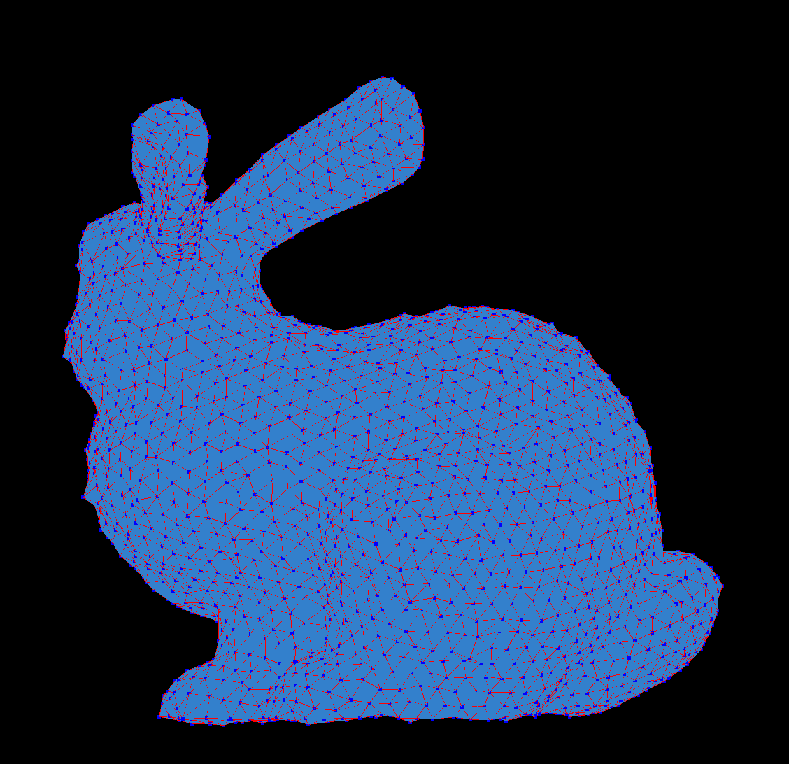
Prototype grid https://github.com/LightningBilly/ACMAlgorithms/blob/master/%E5%9B%BE%E5%BD%A2%E5%AD%A6%E7%AE%97%E6%B3%95/%E4%B8%89%E8%A7%92%E7%BD%91%E6%A0%BC%E7%AE%97%E6%B3%95/MeshWork/src/hw3/bunny_random.obj
Smoothed mesh
https://github.com/LightningBilly/ACMAlgorithms/blob/master/%E5%9B%BE%E5%BD%A2%E5%AD%A6%E7%AE%97%E6%B3%95/%E4%B8%89%E8%A7%92%E7%BD%91%E6%A0%BC%E7%AE%97%E6%B3%95/MeshWork/src/hw3/result.obj
Original model
Smoothed model
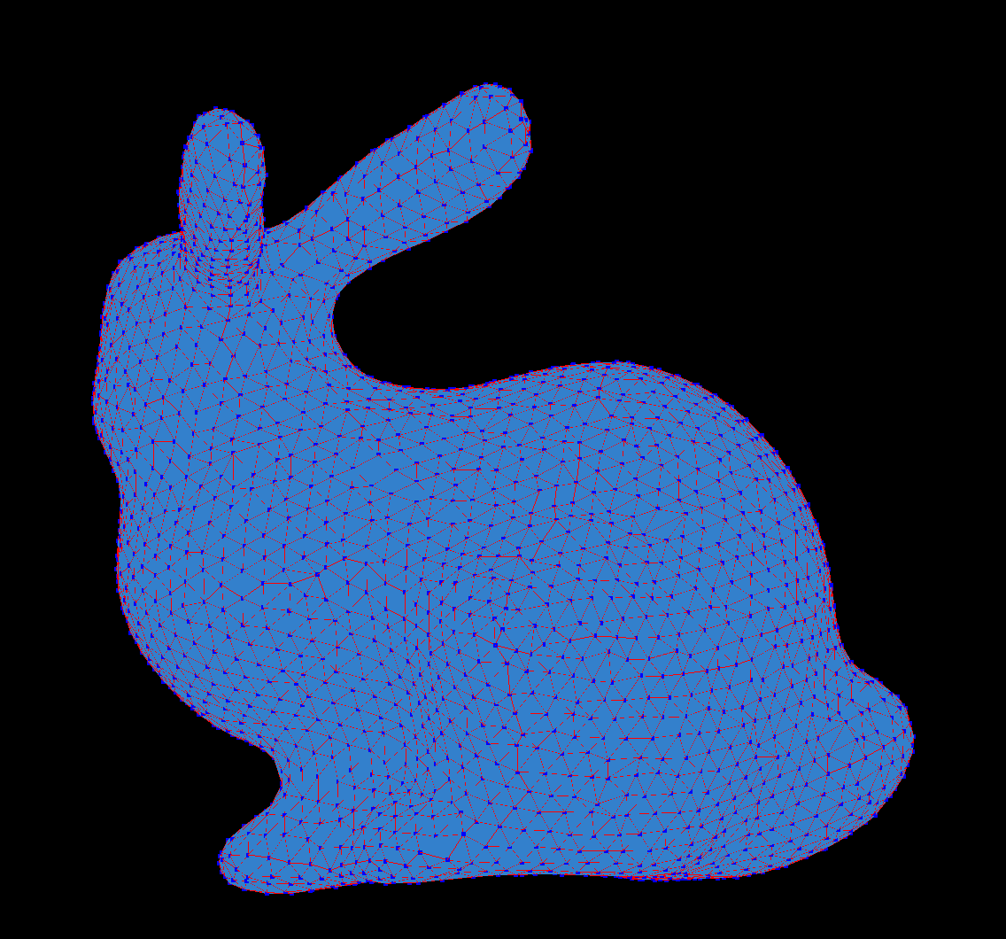
As can be seen from the above figure, there is an obvious smoothing effect.
I hope that through my own sharing, it will be easier for everyone to learn and understand computer knowledge.