1, Introduction
SIFT, scale invariant feature transformation, is a description used in the field of image processing. This description has scale invariance and can detect key points in the image. It is a local feature descriptor.
1. SIFT algorithm features:
(1) It has good stability and invariance, can adapt to the changes of rotation, scale scaling and brightness, and can be free from the interference of angle change, affine transformation and noise to a certain extent.
(2) It has good discrimination, and can match the discrimination information quickly and accurately in the massive feature database
(3) Multiplicity, even if there is only a single object, can produce a large number of feature vectors
(4) High speed, can quickly carry out feature vector matching
(5) Extensibility, which can be combined with other forms of eigenvectors
2 essence of SIFT algorithm
Find the key points in different scale spaces and calculate the direction of the key points.
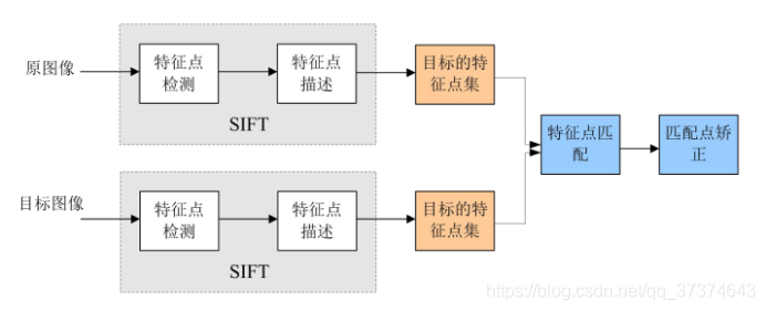
3 the SIFT algorithm realizes feature matching mainly in the following three processes:
(1) Extract key points: key points are some very prominent points that will not disappear due to lighting, scale, rotation and other factors, such as corner points, edge points, bright spots in dark areas and dark spots in bright areas. This step is to search the image position on all scale spaces. Gaussian differential function is used to identify potential points of interest with scale and rotation invariance.
(2) Locate the key points and determine the feature direction: at each candidate position, a fine fitting model is used to determine the position and scale. The selection of key points depends on their stability. Then, one or more directions are assigned to each key position based on the local gradient direction of the image. All subsequent operations on image data are transformed relative to the direction, scale and position of key points, so as to provide invariance to these transformations.
(3) Through the feature vectors of each key point, we can compare them in pairs, find out some matching pairs of feature points, and establish the corresponding relationship between scenes.
4 scale space
(1) Concept
Scale space is the concept and method of trying to simulate human eyes to observe objects in the field of images. For example, when observing a tree, the key is whether we want to observe the leaves or the whole tree: if it is a whole tree (equivalent to observing on a large scale), we should remove the details of the image. If it is a leaf (observed at a small scale), the local details should be observed.
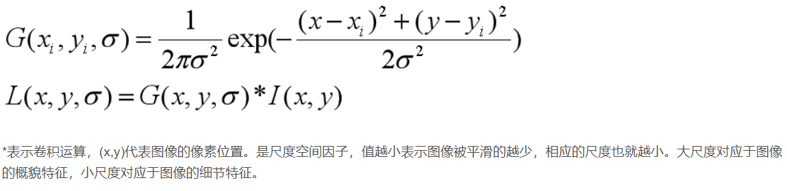
When constructing the scale space, SIFT algorithm adopts Gaussian kernel function for filtering, so that the original image saves the most detailed features. After Gaussian filtering, the detailed features are gradually reduced to simulate the feature representation in the case of large scale.
There are two main reasons for filtering with Gaussian kernel function:
a Gaussian kernel function is the only scale invariant kernel function.
b DoG kernel function can be approximated as LoG function, which can make feature extraction easier. Meanwhile, David In this paper, the author of Lowe proposed that filtering after twice up sampling the original image can retain more information for subsequent feature extraction and matching. In fact, scale space image generation is the current image and different scale kernel parameters σ The image generated after convolution operation.
(2) Express
L(x, y, σ) , Defined as the original image I(x, y) and a variable scale 2-dimensional Gaussian function G(x, y, σ) Convolution operation.
5 construction of Gaussian pyramid
(1) Concept
The scale space is represented by Gaussian pyramid during implementation. The construction of Gaussian pyramid is divided into two steps:
a Gaussian smoothing of the image;
b downsampling the image.
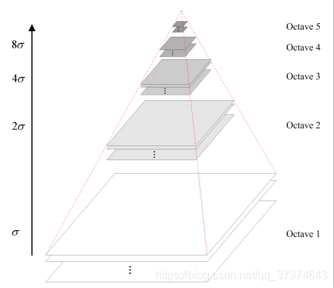
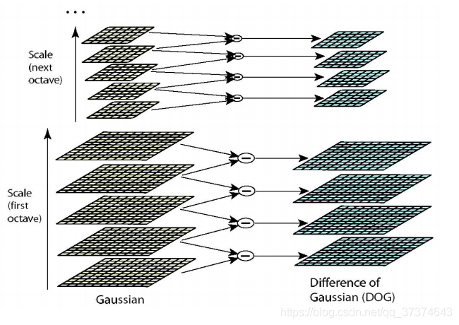
The pyramid model of image refers to the pyramid model that continuously reduces the order and samples the original image to obtain a series of images of different sizes, from large to small and from bottom to top. The original image is the first layer of the pyramid. The new image obtained by each downsampling is one layer of the pyramid (one image per layer), and each pyramid has n layers in total. In order to make the scale reflect its continuity, Gaussian pyramid adds Gaussian filter on the basis of simple downsampling. As shown in the above figure, Gaussian blur is applied to an image of each layer of the image pyramid with different parameters. Octave represents the number of image groups that can be generated by an image, and Interval represents the number of image layers included in a group of images. In addition, during downsampling, the initial image (bottom image) of a group of images on the Gaussian pyramid is obtained by sampling every other point of the penultimate image of the previous group of images.
(2) Express
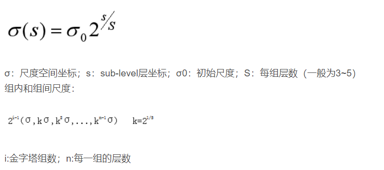
Gaussian image pyramid consists of o groups and s layers
6 DOG space extreme value detection
(1) DOG function
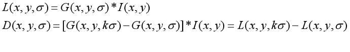
(2) DoG Gaussian difference pyramid
a corresponding to the DOG operator, the DOG pyramid needs to be constructed.
The change of pixel value on the image can be seen through the Gaussian difference image. (if there is no change, there is no feature. The feature must be as many points as possible.) The DOG image depicts the outline of the target.
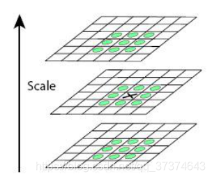
b DOG local extreme value detection
Feature points are composed of local extreme points in dog space. In order to find the extreme point of dog function, each pixel should be compared with all its adjacent points to see whether it is larger or smaller than its adjacent points in image domain and scale domain. Feature points are composed of local extreme points in dog space. In order to find the extreme point of dog function, each pixel should be compared with all its adjacent points to see whether it is larger or smaller than its adjacent points in image domain and scale domain. As shown in the figure below, the detection point in the middle and its 8 adjacent points of the same scale and 9 corresponding to the upper and lower adjacent scales × The two points are compared with 26 points in total to ensure that extreme points are detected in both scale space and two-dimensional image space.
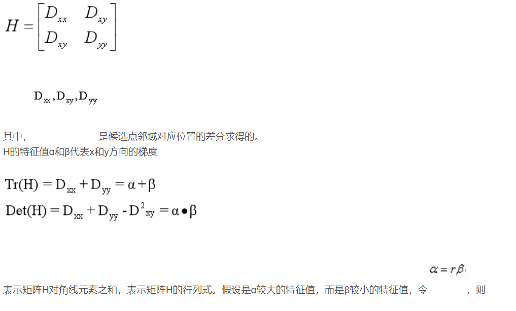
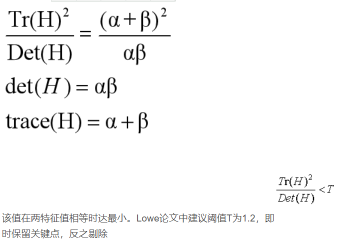
b remove edge effect
In the direction of edge gradient, the principal curvature value is relatively large, while along the edge direction, the principal curvature value is small. Principal curvature and 2 of DoG function D(x) of candidate feature points × 2Hessian matrix is proportional to the eigenvalue of H.
7 key point direction assignment
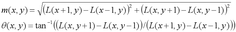
(1) To find the extreme points through scale invariance, we need to use the local features of the image to assign a reference direction to each key point, so that the descriptor is invariant to the rotation of the image. For the key points detected in the DOG pyramid, collect the Gaussian pyramid image 3 σ The gradient and direction distribution characteristics of pixels in the neighborhood window. The modulus and direction of the gradient are as follows:
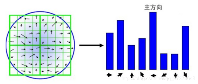
(2) This algorithm adopts the gradient histogram statistical method, which takes the key points as the origin and determines the direction of the key points according to the image pixels in a certain area. After completing the gradient calculation of key points, histogram is used to count the gradient and direction of pixels in the neighborhood. The gradient histogram divides the direction range of 0 ~ 360 degrees into 36 columns, of which each column is 10 degrees. As shown in the figure below, the peak direction of the histogram represents the main direction of the key point, the peak direction of the histogram represents the direction of the neighborhood gradient at the feature point, and the maximum value in the histogram is taken as the main direction of the key point. In order to enhance the robustness of matching, only the direction whose peak value is greater than 80% of the peak value in the main direction is retained as the secondary direction of the key point.
8 key point description
For each key point, it has three information: location, scale and direction. Create a descriptor for each key point and describe the key point with a set of vectors so that it does not change with various changes, such as illumination change, viewing angle change and so on. This descriptor includes not only the key points, but also the pixels around the key points that contribute to it, and the descriptor should have high uniqueness to improve the probability of correct matching of feature points.
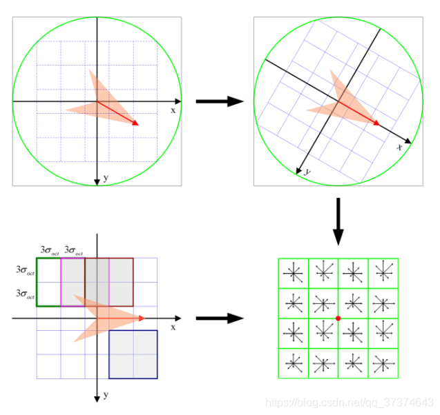
Lowe experimental results show that the descriptor adopts 4 × four × 8 = 128 dimensional vector representation, the comprehensive effect is the best (invariance and uniqueness).
9 key point matching
(1) For template map (reference image) and real-time map (observation map,
observation image) creates a subset of key point descriptions. The target recognition is completed by comparing the key point descriptors in the two-point set. The similarity measure of key descriptor with 128 dimensions adopts Euclidean distance.
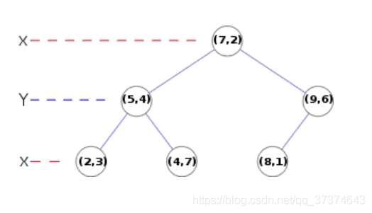
(3) Matching can be completed by exhaustive method, but it takes too much time. Therefore, the data structure of kd tree is generally used to complete the search. The search content is to search the original image feature points closest to the feature points of the target image and the sub adjacent original image feature points based on the key points of the target image.
Kd tree, as shown below, is a balanced binary tree
10 summary
SIFT features have stability and invariance, and play a very important role in the field of image processing and computer vision. It itself is also very complex. Because it is not long to contact sift, we still do not understand the relevant knowledge. After consulting and referring from many parties, the content of this article is not detailed enough. I hope you will forgive me. The following is a rough summary of SIFT algorithm.
(1) Extreme value detection in DoG scale space.
(2) Delete unstable extreme points.
(3) Determine the main direction of feature points
(4) The descriptor of feature points is generated for key point matching.
2, Source code
function varargout = ImageRegistration(varargin)
% IMAGEREGISTRATION MATLAB code for ImageRegistration.fig
%      IMAGEREGISTRATION, by itself, creates a new IMAGEREGISTRATION or raises the existing
%      singleton*.
%
%      H = IMAGEREGISTRATION returns the handle to a new IMAGEREGISTRATION or the handle to
%      the existing singleton*.
%
%      IMAGEREGISTRATION('CALLBACK',hObject,eventData,handles,...) calls the local
%      function named CALLBACK in IMAGEREGISTRATION.M with the given input arguments.
%
%      IMAGEREGISTRATION('Property','Value',...) creates a new IMAGEREGISTRATION or raises the
%      existing singleton*.  Starting from the left, property value pairs are
%      applied to the GUI before ImageRegistration_OpeningFcn gets called.  An
%      unrecognized property name or invalid value makes property application
%      stop.  All inputs are passed to ImageRegistration_OpeningFcn via varargin.
%
%      *See GUI Options on GUIDE's Tools menu.  Choose "GUI allows only one
%      instance to run (singleton)".
%
%

% Edit the above text to modify the response to help ImageRegistration

%

% Begin initialization code - DO NOT EDIT
gui_Singleton = 1;
gui_State = struct('gui_Name',       mfilename, ...
                   'gui_Singleton',  gui_Singleton, ...
                   'gui_OpeningFcn', @ImageRegistration_OpeningFcn, ...
                   'gui_OutputFcn',  @ImageRegistration_OutputFcn, ...
                   'gui_LayoutFcn',  [] , ...
                   'gui_Callback',   []);
if nargin && ischar(varargin{1})
    gui_State.gui_Callback = str2func(varargin{1});
end

if nargout
    [varargout{1:nargout}] = gui_mainfcn(gui_State, varargin{:});
else
    gui_mainfcn(gui_State, varargin{:});
end
% End initialization code - DO NOT EDIT

addpath(pwd);
% --- Executes just before ImageRegistration is made visible.
function ImageRegistration_OpeningFcn(hObject, eventdata, handles, varargin)
% This function has no output args, see OutputFcn.
% hObject    handle to figure
% eventdata  reserved - to be defined in a future version of MATLAB
% handles    structure with handles and user data (see GUIDATA)
% varargin   command line arguments to ImageRegistration (see VARARGIN)5

% Choose default command line output for ImageRegistration
handles.output = hObject;

% eliminate axes Coordinate axis
set(handles.axes1,'Xtick',[],'Ytick',[]);
set(handles.axes1,'Xcolor',[1 1 1],'Ycolor',[1 1 1]);
set(handles.axes2,'Xtick',[],'Ytick',[]);
set(handles.axes2,'Xcolor',[1 1 1],'Ycolor',[1 1 1]);
set(handles.axes3,'Xtick',[],'Ytick',[]);
set(handles.axes3,'Xcolor',[1 1 1],'Ycolor',[1 1 1]);
set(handles.axes4,'Xtick',[],'Ytick',[]);
set(handles.axes4,'Xcolor',[1 1 1],'Ycolor',[1 1 1]);
set(handles.axes5,'Xtick',[],'Ytick',[]);
set(handles.axes5,'Xcolor',[1 1 1],'Ycolor',[1 1 1]);

% Update handles structure
guidata(hObject, handles);

% UIWAIT makes ImageRegistration wait for user response (see UIRESUME)
% uiwait(handles.figure1);


% --- Outputs from this function are returned to the command line.
function varargout = ImageRegistration_OutputFcn(hObject, eventdata, handles)
% varargout  cell array for returning output args (see VARARGOUT);
% hObject    handle to figure
% eventdata  reserved - to be defined in a future version of MATLAB
% handles    structure with handles and user data (see GUIDATA)

% Get default command line output from handles structure
varargout{1} = handles.output;


% --- Executes on button press in pushbutton1.
function pushbutton1_Callback(hObject, eventdata, handles)
% hObject    handle to pushbutton1 (see GCBO)
% eventdata  reserved - to be defined in a future version of MATLAB
% handles    structure with handles and user data (see GUIDATA)
clc
  %%%%%%%%%%%%%%%call OpenImage.m Read in the reference image and obtain the file name and image size%%%
   global Image_I;
   Image_I.FileInformation.IsImage=0;


   while Image_I.FileInformation.IsImage==0
       Image_I1=OpenImage;
    if Image_I.flag ==1
%        delete(Image_I.figure1);
       break;
   end
   end

   if Image_I.flag==0
       delete(Image_I.figure1);
       handles.ImsizeI=Image_I.FileInformation.imsize;
       handles.filenameI=Image_I.FileInformation.filename;
       handles.names_dispI=Image_I.FileInformation.names_disp;
       set(handles.text1,'String',handles.names_dispI);
       guidata(hObject,handles);

       %%%%%%%%%%%%Display reference image
       axes(handles.axes1)
       I=imread(handles.filenameI);
       imshow(I)
   end
% --- Executes on button press in pushbutton2.
function pushbutton2_Callback(hObject, eventdata, handles)
% hObject    handle to pushbutton2 (see GCBO)
% eventdata  reserved - to be defined in a future version of MATLAB
% handles    structure with handles and user data (see GUIDATA)
   clc
  %%%%%%%%call OpenImage.m Read in the floating image and obtain the file name and image size
  global Image_I;
  Image_I.FileInformation.IsImage=0;
  while Image_I.FileInformation.IsImage==0
      Image_J=OpenImage;
    if Image_I.flag ==1
%        delete(Image_I.figure1);
       break;
    end
  end

  if Image_I.flag==0
      delete(Image_I.figure1);
      handles.ImsizeJ=Image_I.FileInformation.imsize;
      handles.filenameJ=Image_I.FileInformation.filename;
      handles.names_dispJ=Image_I.FileInformation.names_disp;
      set(handles.text2,'String',handles.names_dispJ);
      guidata(hObject,handles);


  %%%%%%%%Display floating image%%%%%%%%%%%%%%%%%%%%
  axes(handles.axes2);
  J=imread(handles.filenameJ);
  imshow(J)
  end

% --- Executes on button press in pushbutton3.
function pushbutton3_Callback(hObject, eventdata, handles)
% hObject    handle to pushbutton3 (see GCBO)
% eventdata  reserved - to be defined in a future version of MATLAB
% handles    structure with handles and user data (see GUIDATA)
   clc;
  %%%%%%%%%%%%%%Detect whether the reference image and floating image have been input
  axesIbox=get(handles.axes1,'box');
  axesJbox=get(handles.axes2,'box');
  if strcmp(axesIbox,'off')||strcmp(axesJbox,'off')
      errordlg('Please select Image for Registration','Error');
      error('No Image!');
  end

  %%%%%%%%%%%%%Detect whether the size of the reference image and the floating image are the same
  handles.isSameSizeIJ=strcmp(handles.ImsizeI,handles.ImsizeJ);
  if handles.isSameSizeIJ~=1
      errordlg('Please Select the Same Size Image','Error');
      error('Image Size doesn''t match!');
  end

  %%%%%%%%%%%%Read in and copy images, one for the registration process and the other for output after registration
  BaseImage=imread(handles.filenameI);
  RegisterImage=imread(handles.filenameJ);

  % Realize image registration
  tic
  [img0,diff] = imMosaic(BaseImage,RegisterImage,1);
  toc
  ElapsedTime=toc;
  ElapsedTime=sprintf('Elapsed Time=[%.3f]',ElapsedTime);


  % Display the result after registration
  axes(handles.axes3);
  imshow(img0);
  % Displays the results of the difference
  axes(handles.axes4)
  imshow(diff);

% Set a threshold to eliminate points with inaccurate registration
if numel(size(diff))>2
    diff1 = rgb2gray(diff);
else
    diff1 = diff;
end
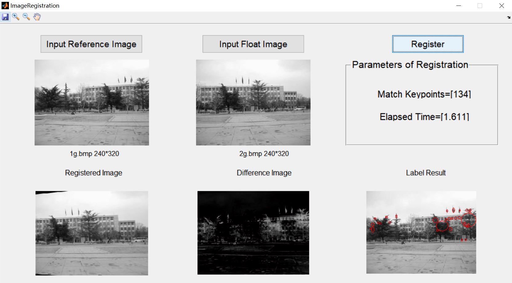
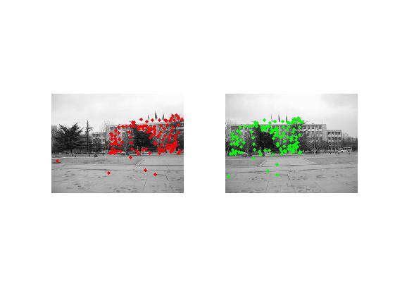
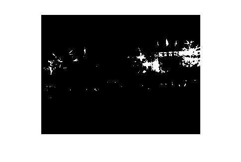
3, Operation results
4, Remarks
Complete code or write on behalf of QQ 1564658423