Abstract: This paper introduces the image classification system based on support vector machine in detail, and gives the algorithm introduction and interface design process of MATLAB. In the interface, you can click to select pictures or folders with pictures, and the system will automatically identify and classify the pictures involved, and you can select your own training model for classification; In addition, the system designs the model training function, which can select the folder of training data set and a small number of selection settings on the interface, and the system can automatically carry out model training, which is suitable for different user-defined data sets; The feature extraction process of the algorithm part adopts the directional gradient histogram (HOG) feature, and the classification process adopts the kernel support vector machine (SVM) algorithm with excellent performance. The system interface is fresh and beautiful. The text contains complete code files and data sets, which can be used out of the box. It is suitable for novice friends to learn and reference.
preface
At present, the algorithm of machine learning has been applied. For the classical support vector machine (SVM) algorithm, it has the characteristics of simple implementation, strong interpretation and superior performance. Nowadays, the research intensity of support vector machine has not decreased. The choice of algorithm should depend on the specific machine learning task. For multi category image classification tasks, support vector machine may be a good choice. The code introduced in this paper can achieve high classification test accuracy, so I want to provide you with a learning Demo for common communication.
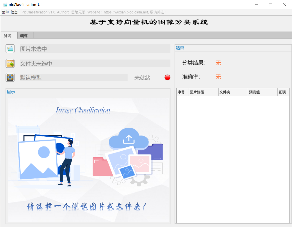
The idea is to develop a script that can classify according to the image content based on the kernel support vector machine (SVM) algorithm. The data set used can be the currently public classified image data set or crawled from the network. In addition to algorithm implementation, in order to facilitate display and training, we use the APP design tool of MATLAB to develop a GUI system interface, which can meet our needs of selecting models, pictures and folder paths. The initial interface is shown in the figure above. In addition, since the self-set data set may be adjusted frequently, the corresponding code also needs to be adjusted. Therefore, the adjustment of the data set is taken into account, and the function of selecting training data set and setting training parameters is designed. Its interface is shown in the figure below.
This paper gives the complete code realized by MATLAB for your reference. The basic readers can reproduce the complete program according to the introduction in the article; For those who want to get all the data sets and program files, you can click the download link provided to get the code that can be run directly. It's not easy to be original, so please give more support. If this article is helpful to you, please like, collect and pay attention!
1. Effect demonstration
(1) Select model + select picture + history
First of all, let's show the effect with the moving picture. After entering the software interface, click the model selection button to pop up the file selection window, where you can select the model file for self training; Then click the picture selection button to select a picture to be tested. After clicking OK, the model will automatically identify the picture content and give the prediction result; The results will be recorded in the table on the right for review and confirmation. The interface of this function is shown in the figure below:
(2) Batch image recognition + classification result display
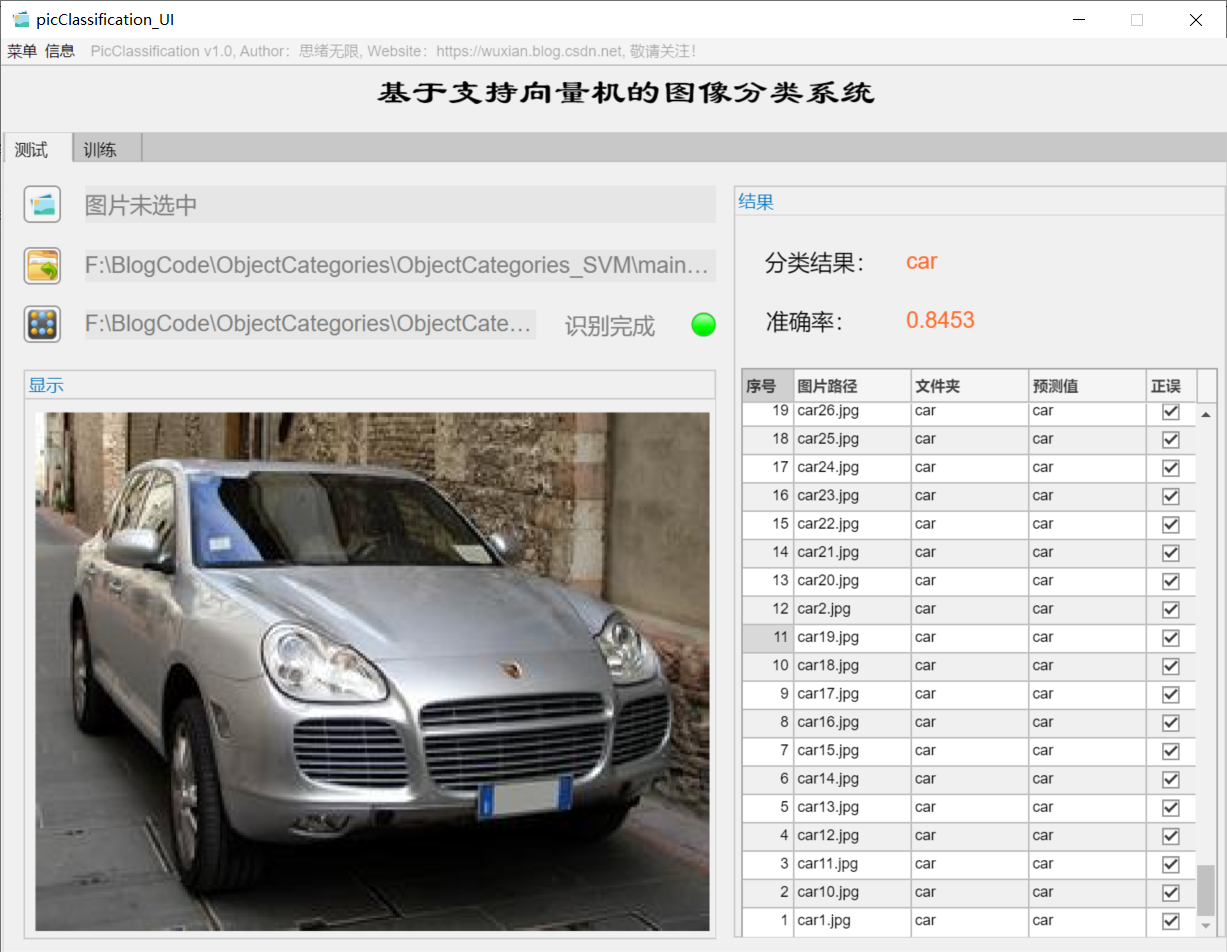
For batch identification, you can select the folder button in the interface and select a picture folder to be tested. The system will automatically identify the files under the folder and classify them. In this process, the recognition results are displayed on the right, including classification results, accuracy and historical records of pictures. Users can click the corresponding serial number in the result record form on the right to look back at the picture and the corresponding recognition result. The demonstration of this part is shown in the following figure:
(3) User defined model training + parameter setting + automatic training
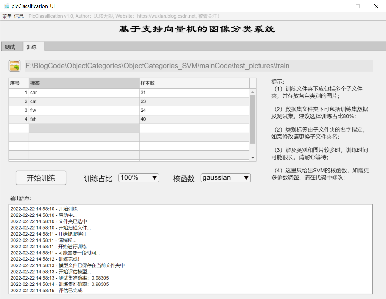
If you want to replace the data set and retrain the model, just click the "training" tab to switch to the training interface. As shown in the figure below, you can select a custom picture folder, which contains multiple subfolders named by category. The system automatically takes the name of the folder as the label of each category, and displays the reading results in the interface. You can select the training settings of training proportion and kernel function, and click "start training" to automatically carry out training. The training process information is displayed on the interface. Finally, you can get the accuracy of training test set and the confusion matrix results of various categories. The model is automatically saved in the current folder for subsequent selection.
2. Caltech 101 dataset
It's easy to think of datasets that mention classification tasks ImageNet , it is undoubtedly a huge training Gallery, which is actually very laborious for us to train and test ourselves (unless you have high-end equipment), so I don't recommend using it in the learning stage. As for the widely used in many earlier papers CIFAR10 / CIFAR100 as well as MNIST Data sets, whose size is too small and their task is relatively simple, are not widely used at present (except water papers). Therefore, the data set we choose here is closer to the real situation Caltech 101 Dataset is also a very popular dataset at present.
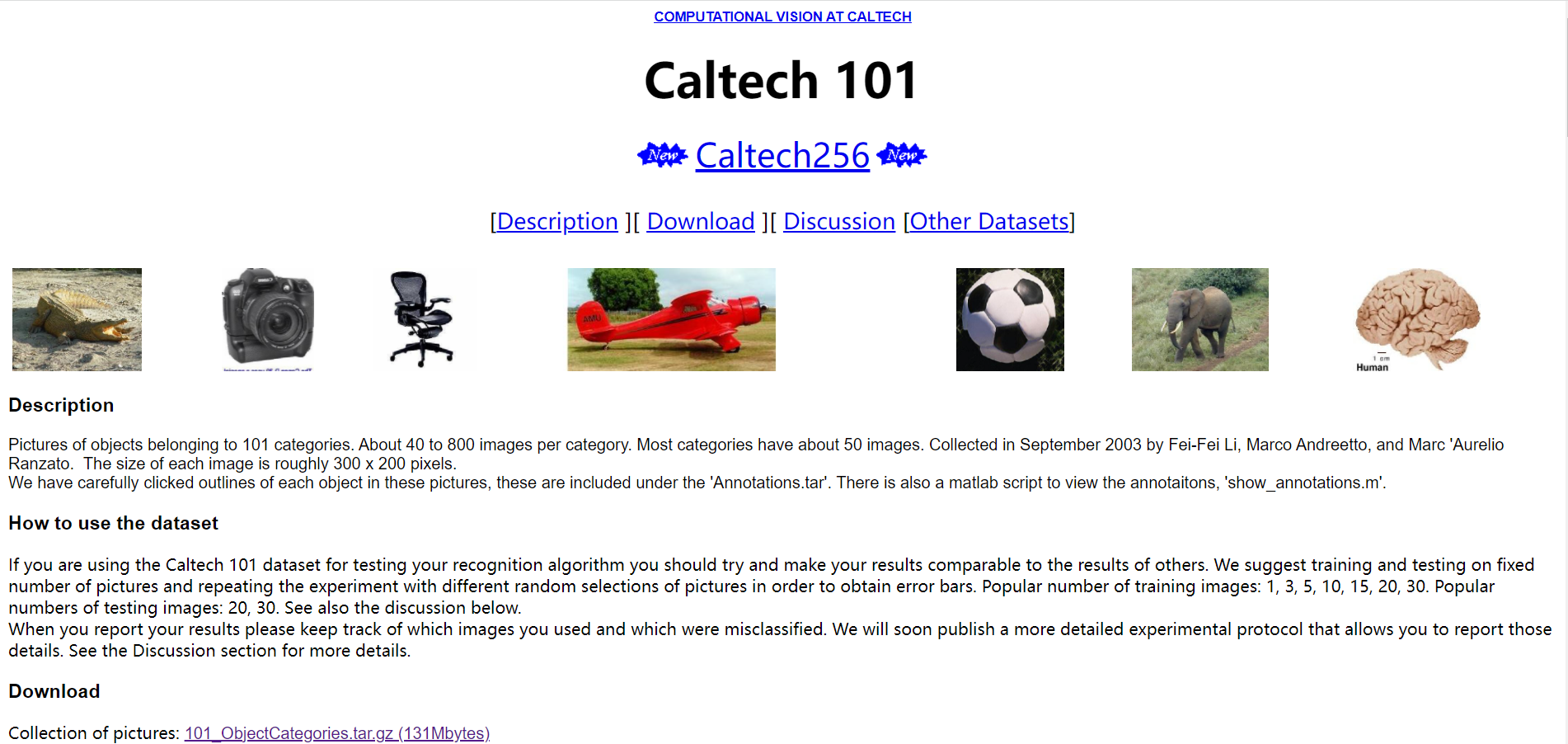
Caltech-101 Dataset It is a data set composed of 101 categories of object pictures. It is mainly used for target recognition and image classification. The official website address is https://www.vision.caltech.edu/Image_Datasets/Caltech101/ . The data set has 40 to 800 pictures in different categories, each picture is 300 * 200 pixels in size, and the publisher of the data set has marked the corresponding target for use. The data set was collected by Li Feifei, mark andreto and Marc'Aurelio Ranzato of California Institute of technology in September 2003. Relevant papers include learning generic visual models from few training examples: an incremental Bayesian approach tested on 101 object categories, one shot learning of object categories, etc.
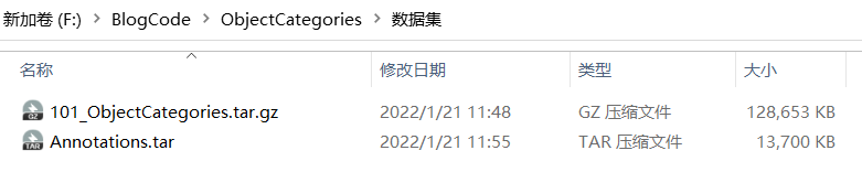
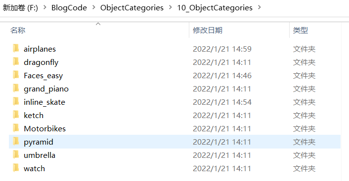
The downloaded dataset file is shown in the figure above. After decompression, you can see that it contains 101 subfolders. Each folder corresponds to a category of pictures, and the name of the folder represents the corresponding label. Due to the large number of data set files, 10 of them are selected here, as shown in the figure below. Copy these folders to the new folder for experiment, and finally determine the data set used.
The dataset is ready and you can now read the pictures through the folder. In MATLAB, the imageDatastore function can be used to conveniently read the picture sets in batches. It scans the folder directory recursively and automatically takes the name of each folder as the label of the image. The code of this part is as follows:
clear
clc
rng default  % Ensure consistent operation of results

mpath = matlab.desktop.editor.getActiveFilename; % Program directory
[pathstr,~]=fileparts(mpath);
cd(pathstr); % Automatically switch to the directory where the program is located

imgDir = fullfile("../10_ObjectCategories/");
% imageDatastore Recursively scan the directory and automatically use each folder name as the label of the image
dataSet = imageDatastore(imgDir, 'IncludeSubfolders', true, 'LabelSource', 'foldernames');
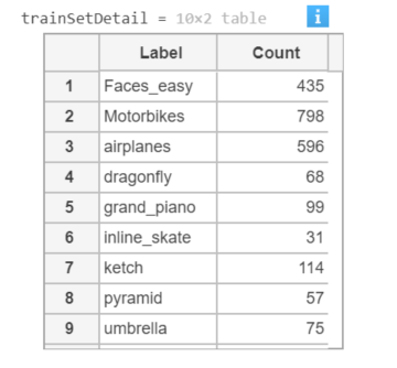
So far, the read data set is stored in the dataSet variable. You can simply view the number of samples of each type of label in the training and test set. The display code is as follows:
trainSetDetail = countEachLabel(dataSet) % Training data
Execute the above code and the results are as follows:
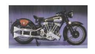
Here is the picture read. The code is as follows:
figure
imshow(dataSet.Files{520});
Execute this code to see the following running results:
Here, we divide the training and test data sets, use the leave one method to use 80% of the data for training, the remaining data for model testing, and save the training and test files in trainset Files and testset In the files variable, the corresponding Label exists in the Label. The code of this part is as follows:
indices = crossvalind('Kfold',dataSet.Labels,5); % Cross validation Division
t=1;

test=(indices == t);
train=~test;
% Training data set
trainSet.Files = dataSet.Files(train);
trainSet.Labels = dataSet.Labels(train);
% Test data set
testSet.Files = dataSet.Files(test);
testSet.Labels = dataSet.Labels(test);
So far, the reading and division of the data set are completed, and then the feature extraction steps are carried out.
3. HOG feature extraction
The real data used to train the classifier is not the original image data, but the feature vector obtained after feature extraction. The feature type used here is HOG, that is, directional gradient histogram. Therefore, the important point here is to correctly extract the HOG features. extractHOGFeatures is the HOG feature extraction function of MATLAB. This function can not only effectively extract features, but also return the visual results of features for easy display. The code of this part is as follows:
cellSize = [4 4];

img = readimage(dataSet, 23);
img = rgb2gray(img);   % Grayscale picture
img = imbinarize(img);
img = imresize(img, [100 100]);
[hog_4x4, vis4x4] = extractHOGFeatures(img,'CellSize',[4 4]);

hogFeatureSize = length(hog_4x4);

% extract HOG features
tStart = tic;

[trainFeatures, trainLabels] = extractHogFromImageSet(trainSet, hogFeatureSize, cellSize); % Feature extraction of training set
[testFeatures, testLabels] = extractHogFromImageSet(testSet, hogFeatureSize, cellSize);    % Test set feature extraction

tEnd = toc(tStart);
fprintf('Time taken to extract features:%.2f second\n', tEnd);
The above code first starts with image grayscale, two value, size adjustment and other preprocessing operations, and then calls the extractHogFromImageSet function to extract the HOG features of training and test sets. Due to the large number of pictures, the feature extraction process still needs some time. Here, the extraction process of training set and test set is timed. Due to the different computing power of the computer, the execution time may be inconsistent, and the time used for feature extraction will be printed finally.
Time taken to extract features: 18.73 second
4. Training and evaluation model
Next, we use the above extracted HOG features to build a support vector machine model, and use the extracted training set features for training. Firstly, the template SVM function is used to construct the template parameters of support vector machine, the gaussian kernel function is selected, the standardized data processing is performed, and the training process is displayed; The fitcecoc function is used to execute the training process, and its code is as follows.
% Training support vector machine
t = templateSVM('SaveSupportVectors',true, 'Standardize', true, 'KernelFunction','gaussian', ...
    'KernelScale', 'auto','Verbose', 0);      % utilize polynomial kernel function, Standardized processing of data and display of training process( verbose (cancel display when taking 0)

tStart = tic; % Timing start
classifier = fitcecoc(trainFeatures, trainLabels, 'Learner', t); % train SVM Model
tEnd = toc(tStart);
fprintf('Training model time:%.2f second\n', tEnd);
After the training is completed, we can use the trained classifier to predict. Here, we first use the test set evaluation model and calculate the classification evaluation index. The code for predicting the test set is as follows:
tStart = tic;
% Predict the test data set
predictedLabels = predict(classifier, testFeatures);
tEnd = toc(tStart);
fprintf('Time taken by the model to predict the test set:%.2f second\n', tEnd);
The operation results are as follows:
Time taken by the model to predict the test set: 5.75 second
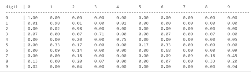
After the prediction results are obtained, the confusion matrix can be used to evaluate the results. The following code first calculates the confusion matrix results, and then prints the results:
The classification accuracy can be calculated by the following code:
accuracy = sum(predictedLabels == testLabels) / numel(testLabels);
fprintf('Accuracy of the model on the test set:%.0f%%\n', accuracy*100);
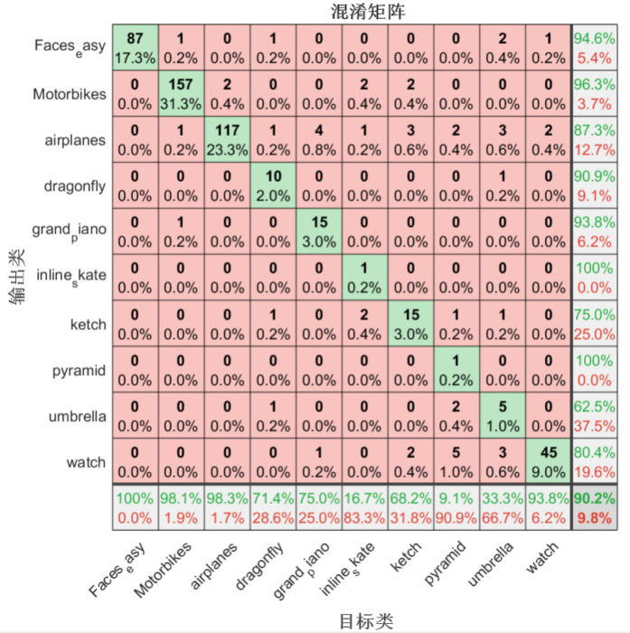
The above code shows the results of the confusion matrix, but it may not be intuitive enough. Draw the confusion matrix diagram below to help better understand the model performance:
% Draw confusion matrix
plotconfusion(testLabels, predictedLabels);
After running the code, the confusion matrix is displayed as shown in the figure below. The grid (green grid) on the diagonal of each line shows the correct number and proportion of a certain type of sample prediction. The grid in the lower right corner represents the classification accuracy. It can be seen that the classifier has an overall classification accuracy of 90.2%.
In order to facilitate the subsequent test, the model file is saved here, and its code is as follows:
save('trainedSvmModel.mat','classifier');
5. Test model
Here we select several pictures to test, so as to have a more intuitive feeling of the effect of the model. The code of this part is as follows:
clear
clc
rng default  % Ensure consistent operation of results
img_test_1 = imread("../10_ObjectCategories/airplanes/image_0137.jpg");
img_test_2 = imread("../10_ObjectCategories/dragonfly/image_0001.jpg");
img_test_3 = imread("../10_ObjectCategories/inline_skate/image_0003.jpg");
img_test_4 = imread("../10_ObjectCategories/ketch/image_0005.jpg");
img_test_5 = imread("../10_ObjectCategories/Motorbikes/image_0006.jpg");
img_test_6 = imread("../10_ObjectCategories/umbrella/image_0010.jpg");
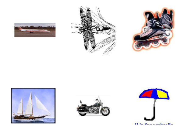
After reading the pictures, first use imshow function to display several pictures, and use subplot function to divide the picture coordinate axis area, so as to display six pictures:
figure;
subplot(2, 3, 1); imshow(img_test_1);
subplot(2, 3, 2); imshow(img_test_2);
subplot(2, 3, 3); imshow(img_test_3);
subplot(2, 3, 4); imshow(img_test_4);
subplot(2, 3, 5); imshow(img_test_5);
subplot(2, 3, 6); imshow(img_test_6);
Execute the above code, and the running results are shown in the following figure:
Similar to the previous chapter, first extract the HOG feature. Here, visually display the extracted feature and compare it with the original image. The code is as follows:
img = rgb2gray(img_test_1);
img = imbinarize(img);
% img = imresize(img, [100 100]);
[hog_1, vis_1] = extractHOGFeatures(img,'CellSize',[4 4]);
figure
subplot(2,1,1);
imshow(img_test_1)
title("original image ")
subplot(2, 1, 2)
plot(vis_1);
title("Feature image")
Run the above code, and the image operation result of feature extraction is shown in the following figure:

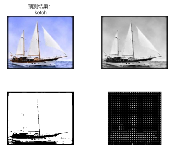
Next, we load the previously trained model, predict the read pictures and display the results. It is worth noting that the preprocessing work of each picture before prediction is to visualize the results of grayscale, binarization and HOG features in the same drawing window through the code. The code is as follows:
load("trainedSvmModel.mat", "classifier");
img_gray = rgb2gray(img_test_4);
img_bin = imbinarize(img_gray);
img = imresize(img_bin, [100 100]);
[hog_4, vis_4]  = extractHOGFeatures(img,'CellSize',[4 4]);

% Predict the test data set
fea_4 = extractHOGFeatures(img,'CellSize',[4 4]);
predictedLabels = predict(classifier, fea_4);
fprintf("Prediction results:%s",predictedLabels);

figure
subplot(2,2,1)
imshow(img_test_4);
title(["Prediction results:", char(predictedLabels)])
subplot(2,2,2)
imshow(img_gray);

subplot(2,2,3)
imshow(img_bin);
subplot(2,2,4)
plot(vis_4)
Run the above code and the display results are as follows:
Download link
If you want to obtain all the program files involved in the blog (including data set, m, UI files, etc., as shown in the figure below), it has been packaged and uploaded to the blogger's bread multi platform and CSDN download resources. This resource has been uploaded to bread multi website and CSDN download resource channel, which can be obtained by clicking the following link. All involved files have been packaged in it at the same time, and click to run. The screenshot of the complete file is as follows:
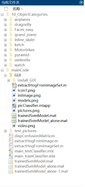
The resources under the folder are shown as follows:
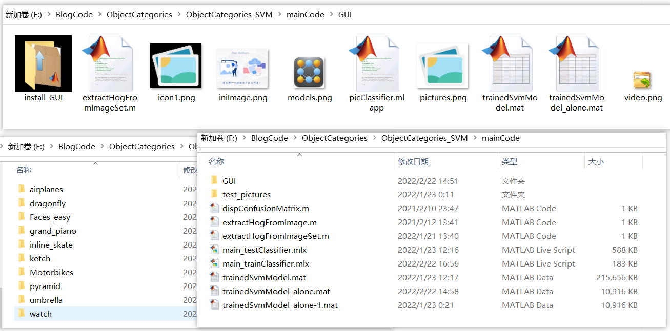
Note: this resource has been debugged and can be run through MATLAB R2021b after downloading; The main training program is main_trainClassifier.mlx, the test program can run main_testClassifier.mlx, to use the GUI interface, run picclassifier Mlapp file; Most of other program files are functions rather than scripts that can be run directly. Do not click run directly when using! ➷➷➷
Full resource download link 1: Blogger's complete resource download page on bread multi website
Full resource download link 2: https://mianbaoduo.com/o/bread/mbd-YpiTl5ht
Note: the above two links are bread multi platform download links, and the download link of CSDN download resource channel will be uploaded later.
Concluding remarks
Due to the limited ability of bloggers, even if the methods mentioned in the blog have been tested, there will inevitably be omissions. I hope you can enthusiastically point out the mistakes so that you can present them in front of you in a more perfect and rigorous manner when you modify them next time.