1 Introduction

Facial expression recognition technology involves the research fields of emotion computing, image processing, machine vision, pattern recognition, biometric recognition and so on This paper introduces a facial expression recognition technology based on lpq feature and support vector machine (SVM)

In this experiment, SVM (support vector machine) classifier, which is very popular in recent years, is used. The work of classifier is divided into two steps: training and testing. First learn the samples, pre judge the samples, learn and classify the extracted feature vectors, and then classify the test objects through the classifier. For this experiment, face recognition is realized. The traditional classifier only considers the fitting of training samples, aims to minimize the classification errors on the training set, and improves the recognition rate of the classifier on the test set by providing sufficient training samples. Therefore, when the training samples are limited, that is, when the training samples are small, the traditional classifier can not guarantee the effective classification accuracy. The classification idea of SVM is based on structural risk minimization, taking into account the minimization of training error and test error, which is embodied in the selection of classification model and model parameters. It can effectively ensure the classification accuracy in small sample problems. The idea of nonlinear SVM (non linear support vector machine) is to find a mapping space from low dimension to high dimension, so that the features that are not easy to distinguish in the original low dimension space can be projected into the high dimension space to make it more separable. When the hyperplane of support vector machine is solved in the high-dimensional feature space and projected back to the original low-dimensional space, it presents a nonlinear surface, so it is called nonlinear support vector machine. The key of nonlinear support vector machine is how to map from low dimension to high dimension. This mapping relationship is called kernel function, which theoretically needs to meet Mercer theorem (any positive semidefinite function can be used as kernel function). This paper uses the current mainstream RBF (radial basis function kernel), that is, the support vector machine classifier based on RBF is realized.

Part 2 code

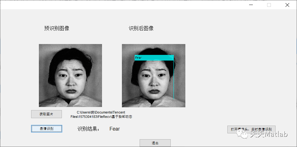
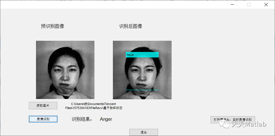
% Input parameter description: img For picture information, winSize Is the window size, decorr To indicate whether to use an inverse relationship, freqestim To indicate which method to use for local frequency estimation, mode Define output format for% Output parameter description: LPQdesc by LPQ Characteristic calculation results% Function function: LPQ Characteristic calculation​function LPQdesc = lpq(img,winSize,decorr,freqestim,mode)​​%% Default parameters% Window size if nargin<2 || isempty(winSize)    winSize=3; % Default window size 3 end​% Decorrelation if nargin<3 || isempty(decorr)       decorr=1; % Decorrelation used by default endrho=0.90; % Using correlation coefficientρ= 0.9 Default​% Local frequency estimation (frequency point)[α，0 ]，[ 0 ]，[α，α，α]，and[α，α])if nargin<4 || isempty(freqestim)    freqestim=1; %Using short-time Fourier transform( STFT)With uniform window default endSTFTalpha=1/winSize;  % stay STFT methodα(Gaussian derivativeα= 1)sigmaS=(winSize-1)/4; % Gaussian window for short-time Fourier transformσ(If freqestim = = 2)sigmaA=8/(winSize-1); % Orthogonal filter of Gaussian derivative∑(If freqestim = = 3)​% Output mode if nargin<5 || isempty(mode)    mode='nh'; % Normalized histogram returned as default end​% other convmode='valid'; %In the calculation part, there are sufficient neighbors to describe the response. If all pixels using "same" are included (inferred image zero).​​%% Check inputsif size(img,3)~=1    error('Only gray scale image can be used as input');%The only grayscale image can be used as input endif winSize<3 || rem(winSize,2)~=1   error('Window size winSize must be odd number and greater than equal to 3');%winSize Is an odd window size greater than or equal to 3 endif sum(decorr==[0 1])==0    error('decorr parameter must be set to 0->no decorrelation or 1->decorrelation. See help for details.');%decorr The parameter must be set to 0 or 1 &gt; &gt;No decoherence decorrelation. See help for details endif sum(freqestim==[1 2 3])==0    error('freqestim parameter must be 1, 2, or 3. See help for details.');%freqestim Parameter must be 1, 2, or 3. See help for details endif sum(strcmp(mode,{'nh','h','im'}))==0    error('mode must be nh, h, or im. See help for details.');%Mode must NH，H，or IM. See help for details end​​%% Initializeimg=double(img); % Image conversion to doubler=(winSize-1)/2; % Window size radius x=-r:r; % Spatial coordinates of the form u=1:r; % Coordinates of positive half form in frequency domain (required for Gaussian derivative)​%% Form 1-D filters Form 1-D wave filter if freqestim==1 % STFT Uniform window    %Basic STFT wave filter    w0=(x*0+1);    w1=exp(complex(0,-2*pi*x*STFTalpha));    w2=conj(w1);end​​%%Run the filter to calculate the frequency response at four points. Real and imaginary parts stored separately% Run first filter Run the filter first filterResp=conv2(conv2(img,w0.',convmode),w1,convmode);% Frequency domain matrix four frequency coordinates (real and imaginary parts of each frequency) freqResp=zeros(size(filterResp,1),size(filterResp,2),8); % Storage filter output freqResp(:,:,1)=real(filterResp);freqResp(:,:,2)=imag(filterResp);% For procedures repeated at other frequencies filterResp=conv2(conv2(img,w1.',convmode),w0,convmode);freqResp(:,:,3)=real(filterResp);freqResp(:,:,4)=imag(filterResp);filterResp=conv2(conv2(img,w1.',convmode),w1,convmode);freqResp(:,:,5)=real(filterResp);freqResp(:,:,6)=imag(filterResp);filterResp=conv2(conv2(img,w1.',convmode),w2,convmode);freqResp(:,:,7)=real(filterResp);freqResp(:,:,8)=imag(filterResp);​% Reading frequency matrix size[freqRow,freqCol,freqNum]=size(freqResp);​%% If decorrelation is applied, the covariance matrix and the corresponding whitening transformation are calculated if decorr == 1    % Calculate the covariance matrix (pixel position between covariances) x_i and x_j yes Rho ^ | | x_i-x_j | |)    [xp,yp]=meshgrid(1:winSize,1:winSize);    pp=[xp(:) yp(:)];    dd=dist(pp,pp');    C=rho.^dd;        % Form a two-dimensional filter Q1，Q2，Q3，Q4 And the corresponding two-dimensional matrix operator M(Separated real and imaginary parts)    q1=w0.'*w1;    q2=w1.'*w0;    q3=w1.'*w1;    q4=w1.'*w2;    u1=real(q1); u2=imag(q1);    u3=real(q2); u4=imag(q2);    u5=real(q3); u6=imag(q3);    u7=real(q4); u8=imag(q4);    M=[u1(:)';u2(:)';u3(:)';u4(:)';u5(:)';u6(:)';u7(:)';u8(:)'];        % Calculate whitening transformation matrix V    D=M*C*M';    A=diag([1.000007 1.000006 1.000005 1.000004 1.000003 1.000002 1.000001 1]); % Use "random" (almost unit) diagonal matrix to avoid multiple eigenvalues.Use "random" (basic cell) to avoid multiple eigenvalue diagonal matrices      [U,S,V]=svd(A*D*A);       % Reshaped frequency response    freqResp=reshape(freqResp,[freqRow*freqCol,freqNum]);​    % Perform whitening transformation    freqResp=(V.'*freqResp.').';        % e Undo reshape    freqResp=reshape(freqResp,[freqRow,freqCol,freqNum]);end​​%% Quantification and calculation LPQ Codeword LPQdesc=zeros(freqRow,freqCol); % Initialization code word( LPQ Image size (depending on availability or use in the same region) for i=1:freqNum    LPQdesc=LPQdesc+(double(freqResp(:,:,i))>0)*(2^(i-1));end​%% Card exchange format LPQ Output of encoded image if strcmp(mode,'im')    LPQdesc=uint8(LPQdesc);end​%% If required histogram if strcmp(mode,'nh') || strcmp(mode,'h')    LPQdesc=hist(LPQdesc(:),0:255);end​%% Histogram specification if required if strcmp(mode,'nh')    LPQdesc=LPQdesc/sum(LPQdesc);end​​​​​

3 simulation results

4 references

[1] Huang Mingwei Facial expression recognition algorithm based on principal component analysis and support vector machine [J] Computer knowledge and technology: Academic Edition, 2013, 9 (7): 3

Blogger profile: good at matlab simulation in intelligent optimization algorithm, neural network prediction, signal processing, cellular automata, image processing, path planning, UAV and other fields. Relevant matlab code problems can be exchanged through private letters.

Some theories cite online literature. If there is infringement, contact the blogger and delete it.