Despite the recent success of long tail target detection, almost all long tail target detectors are developed based on the two-stage paradigm. In practice, one-stage detectors are more common in the industry because they have a simple and fast Pipeline and are easy to deploy. However, in the case of long tail, this work has not been explored so far.
In this paper, we study whether the one-stage detector performs well in this case. The author found that the main obstacle to the excellent performance of one-stage detector is that there are different degrees of positive and negative imbalance in the category under the long tail data distribution. The traditional Focal Loss balances the training process with the same modulation factor in all categories, so it can not deal with the long tail problem.
In order to solve this problem, this paper proposes balanced Focal Loss(EFL), which independently rebalances the loss contribution of different categories of samples according to the imbalance degree of positive and negative samples of different categories. Specifically, EFL adopts a category related modulation factor, which can be dynamically adjusted according to the training status of different categories. A large number of experiments on the challenging LVISv1 benchmark prove the effectiveness of the proposed method. Through end-to-end training, EFL achieved 29.2% of the total AP and achieved significant performance improvement in rare categories, surpassing all the existing state-of-the-art methods.
Open source address: https://github.com/ModelTC/EOD
1 Introduction
Long tail target detection is a challenging task, which has attracted more and more attention in recent years. In the long tail scenario, the data usually has a Zipfian distribution (such as LVIS), in which several header classes contain a large number of instances and dominate the training process. In contrast, a large number of tail classes lack instances and therefore perform poorly. The common solutions of long tail target detection are data resampling, decoupling training and loss reweighting. Despite the success in alleviating the long tail imbalance, almost all long tail object detectors are developed based on the two-stage method extended by R-CNN. In practice, one-stage detectors are more suitable for real scenes than two-stage detectors because they are computationally efficient and easy to deploy. However, there is no relevant work in this regard.
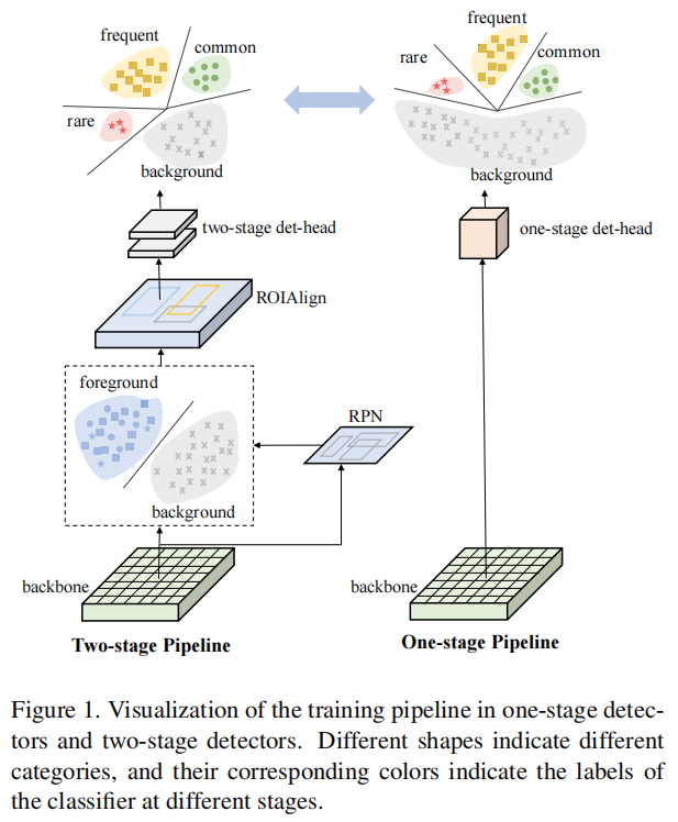
Compared with the two-stage method including regional suggestion network (RPN), which filters out most background samples before providing suggestions to the final classifier, the one-stage detector directly detects targets on the regular and dense candidate location set. As shown in Figure 1, due to the dense prediction mode, extreme Foreground Background imbalance is introduced into the one-stage detector. Combined with the imbalance of foreground categories (i.e. foreground samples of categories) in the long tail scenario, the performance of the one-stage detector is seriously damaged.
Focal Loss is a conventional solution to the problem of foreground background imbalance. It focuses on the learning of hard foreground samples and reduces the influence of simple background samples. This loss redistribution technique works well in the case of balanced distribution of categories, but it is not enough to deal with the imbalance between prospect categories in the case of long tail. In order to solve this problem, the author starts with the existing solutions in the two stages (such as EQLv2), and adjusts them to deal with Focal Loss together in the one-stage detector. The authors found that these solutions brought only minor improvements compared with their application in two-stage detectors (see Table 1). Then, the author believes that simply combining the existing solutions with Focal Loss can not solve these two types of imbalance problems at the same time. By comparing the ratio of positive samples to negative samples in different data distributions (see Figure 2), it is further recognized that the essence of these imbalance problems is the inconsistency of the degree of positive and negative imbalance between categories. Rare categories suffer from more serious positive and negative imbalances than frequent categories, so more attention is needed.
In this paper, an equalization Focal Loss(EFL) is proposed by introducing a class related modulation factor into Focal Loss. The modulation factor with two decoupled dynamic factors (i.e. focusing factor and weighting factor) independently deals with different types of positive and negative imbalances. Focusing factor determines the learning concentration of hard samples according to the imbalance degree of the corresponding categories of hard samples. The weighting factor increases the influence of rare categories and ensures that the loss contribution of rare samples will not be submerged by frequent samples. The synergy of these two factors enables EFL to uniformly overcome the foreground background imbalance and foreground category imbalance when applying one-stage detector in long tail scenes.
Extensive experiments have been carried out on the challenging LVISv1 benchmark. Through simple and effective initial training, 29.2% AP is achieved, which exceeds the existing long tail target detection methods. Experimental results on open images also demonstrate the generalization ability of the method.
To sum up, the main contributions can be summarized as follows:
- It is the first work to study single-stage long tail target detection;
- A new equalization Focal Loss is proposed, which extends the original Focal Loss with a class related modulation factor. It is a generalized Focal Loss form, which can solve the problems of foreground background imbalance and foreground category imbalance at the same time;
- Extensive experiments are carried out on LVISv1 benchmark, and the results show the effectiveness of the method. It establishes a new advanced technology, which can be well applied to any single-stage detector.
Related work
2.1 common target detection
In recent years, due to the great success of convolutional neural network, the computer vision community has made remarkable progress in target detection. Modern target detection framework can be roughly divided into two-stage method and one-stage method.
1. Two stage target detection
With the emergence of fast RCNN, two-stage method plays a leading role in modern target detection. The two-stage detector first generates target suggestions through regional suggestion mechanism (such as selective search or RPN), and then performs spatial extraction of feature map according to these suggestions for further prediction. Due to this recommendation mechanism, a large number of background samples are filtered out. After that, the classifiers of most two-stage detectors are trained on the relatively balanced distribution of foreground and background samples, with a ratio of 1:3.
2. One stage target detection
Generally speaking, the one-stage target detector has a simple and fast training pipeline, which is closer to real-world applications. In a single-stage scenario, the detector predicts the detection frame directly from the feature map. The classifier of one-stage target detector is trained on a dense set of about 104 to 105 candidate samples, but only a few candidate samples are foreground samples. Some studies try to solve the extreme Foreground Background imbalance problem from the perspective of difficult sample mining or more complex resampling / reweighting schemes.
Focal Loss and its derivatives reshape the standard cross entropy loss, so as to reduce the loss assigned to well classified samples, and focus on the training of hard samples. Benefiting from Focal Loss, the one-stage target detector achieves the performance very close to the two-stage target detector method, and has higher reasoning speed. Recently, some scholars have tried to improve the performance from the perspective of label allocation.
The EFL proposed in this paper can be well applied to these single-stage frameworks and bring significant performance improvement in the long tail scenario.
2.2 long tailed target detection
Compared with general target detection, long tail target detection is a more complex task because of the extreme imbalance between foreground categories. A direct way to solve this imbalance is to perform data resampling during training. Repetitive factor sampling (RFS) oversamples the training data from the tail class and the training data from the head class at the image level.
Some scholars train the detector in a decoupled way, and propose an additional classification branch with class balanced sampler from the instance level. Forest R-CNN resampling from RPN with different NMS thresholds is recommended. Other work is to realize data resampling through meta learning or memory enhancement.
Loss reweighting is another widely used solution to solve the long tail distribution problem. Some researchers have proposed equilibrium loss (EQL), which reduces the gradient suppression of head class to tail class. EQLv2 is an upgraded version of EQL. It adopts a new gradient guidance mechanism to re measure the loss contribution of each category.
Some scholars have also explained the long tail distribution problem from the perspective of non statistics, and proposed adaptive class suppression loss (ACSL). DisAlign proposes a generalized reweighting method, which introduces a balance class before loss design. In addition to data resampling and loss reweighting, many excellent works have been tried from different angles, such as decoupling training, edge modification, incremental learning and causal reasoning.
However, all these methods are developed with two-stage target detector. So far, there is no related work on single-stage long tail target detection. This paper presents the first solution of long tail target detection based on single stage. It simply and effectively goes beyond all existing methods.
3. This method
3.1 focus loss
In the one-stage target detector, Focal Loss is the solution to the foreground background imbalance problem. It redistributes the loss contribution of easy samples and difficult samples, and greatly weakens the influence of most background samples. The formula of Focal Loss of class II is:
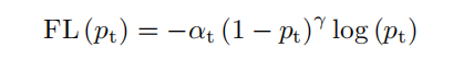
Represents the prediction confidence score of a candidate target, and the term is a parameter that balances the importance of positive samples and negative samples. Regulatory factors are a key component of Focal Loss. By predicting scores and Focal parameters, the loss of simple samples is reduced, focusing on the learning of difficult samples.
A large number of negative samples are easy to classify, while positive samples are usually difficult to classify. Therefore, the imbalance between positive samples and negative samples can be roughly regarded as the imbalance between easy samples and difficult samples. The Focal parameter determines the influence of Focal Loss. It can be concluded from the equation that a large will greatly reduce the loss contribution of most negative samples, thus improving the impact of positive samples. This conclusion shows that the higher the degree of imbalance between positive and negative samples, the greater the expected value of.
When multi class cases are involved, Focal Loss is applied to C classifiers, which act on the output log of s-type function transformation of each instance. C is the number of categories, which means that a classifier is responsible for a specific category, that is, a binary classification task. Since Focal Loss also treats all categories of learning with the same modulation factor, it fails to deal with the long tail imbalance problem (see Table 2).
3.2 Equalized Focal Loss
In the long tail dataset (LVIS), in addition to the foreground background imbalance, the classifier of one-stage detector also has the imbalance between foreground categories.
As shown in Figure 2, if viewed from the y-axis, the ratio of positive samples to negative samples is far less than zero, which mainly reveals the imbalance between foreground and background samples. Here, the value of this ratio is called positive and negative imbalance. From the perspective of x-axis, it can be seen that there are great differences in the degree of imbalance between different categories, indicating the imbalance between prospect categories.
Obviously, in the data distribution (i.e. COCO), the degree of imbalance of all categories is similar. Therefore, it is sufficient for Focal Loss to use the same modulation factor. On the contrary, the degree of these imbalances is different in the case of long tail data. Rare categories suffer from more severe positive and negative imbalances than common categories. As shown in Table 1. Most one-stage detectors perform worse in rare categories than in frequent categories. This shows that the same modulation factor is not applicable to all different degrees of imbalance.
1,Focusing Factor
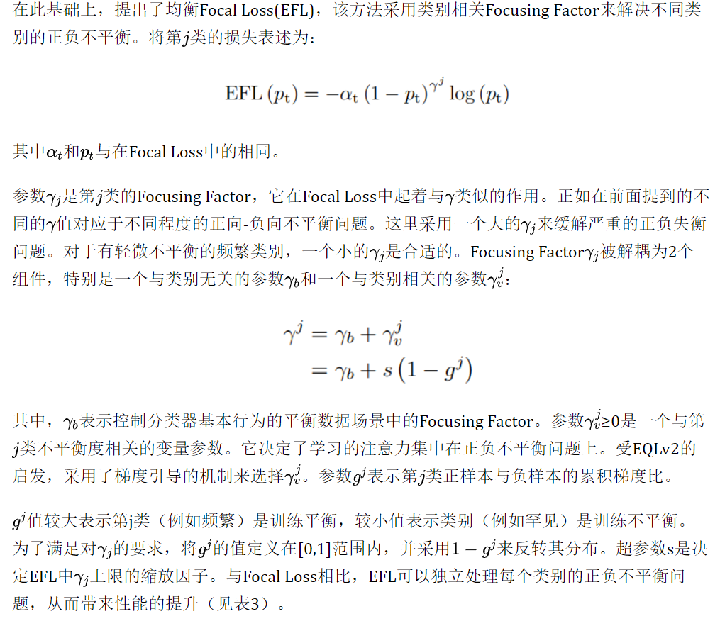
2,Weighting Factor
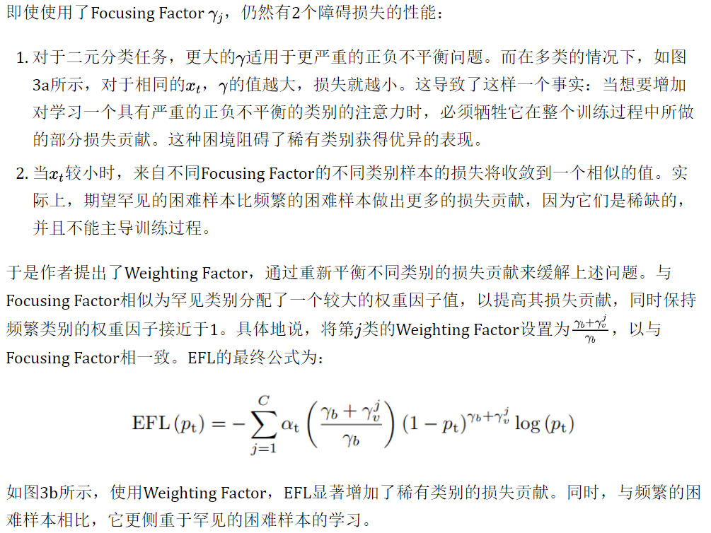
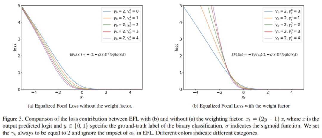
Focusing Factor and Weighting Factor constitute the category related regulatory factors of EFL. It enables the classifier to dynamically adjust the loss contribution of samples according to the training state of samples and the corresponding category state. Both Focusing Factor and Weighting Factor play an important role in EFL. Meanwhile, in the balanced data distribution, all EFLS are equivalent to Focal Loss. This attractive feature enables EFL to be well applied to different data distributions and data samplers.
PyTorch is implemented as follows:
@LOSSES_REGISTRY.register('equalized_focal_loss')
class EqualizedFocalLoss(GeneralizedCrossEntropyLoss):
    def __init__(self,
                 name='equalized_focal_loss',
                 reduction='mean',
                 loss_weight=1.0,
                 ignore_index=-1,
                 num_classes=1204,
                 focal_gamma=2.0,
                 focal_alpha=0.25,
                 scale_factor=8.0,
                 fpn_levels=5):
        activation_type = 'sigmoid'
        GeneralizedCrossEntropyLoss.__init__(self,
                                             name=name,
                                             reduction=reduction,
                                             loss_weight=loss_weight,
                                             activation_type=activation_type,
                                             ignore_index=ignore_index)

        # Hyper parameter of Focal Loss
        self.focal_gamma = focal_gamma
        self.focal_alpha = focal_alpha

        # ignore bg class and ignore idx
        self.num_classes = num_classes - 1

        # Hyperparameters of EFL loss function
        self.scale_factor = scale_factor
        # Initialize the gradient variable of positive and negative samples
        self.register_buffer('pos_grad', torch.zeros(self.num_classes))
        self.register_buffer('neg_grad', torch.zeros(self.num_classes))
        # Initialize positive and negative sample variables
        self.register_buffer('pos_neg', torch.ones(self.num_classes))

        # grad collect
        self.grad_buffer = []
        self.fpn_levels = fpn_levels

        logger.info("build EqualizedFocalLoss, focal_alpha: {focal_alpha}, focal_gamma: {focal_gamma},scale_factor: {scale_factor}")

    def forward(self, input, target, reduction, normalizer=None):
        self.n_c = input.shape[-1]
        self.input = input.reshape(-1, self.n_c)
        self.target = target.reshape(-1)
        self.n_i, _ = self.input.size()

        def expand_label(pred, gt_classes):
            target = pred.new_zeros(self.n_i, self.n_c + 1)
            target[torch.arange(self.n_i), gt_classes] = 1
            return target[:, 1:]

        expand_target = expand_label(self.input, self.target)
        sample_mask = (self.target != self.ignore_index)

        inputs = self.input[sample_mask]
        targets = expand_target[sample_mask]
        self.cache_mask = sample_mask
        self.cache_target = expand_target

        pred = torch.sigmoid(inputs)
        pred_t = pred * targets + (1 - pred) * (1 - targets)
  # map_val is: 1-g^j
        map_val = 1 - self.pos_neg.detach()
        # dy_gamma is: gamma^j
        dy_gamma = self.focal_gamma + self.scale_factor * map_val

        # focusing factor
        ff = dy_gamma.view(1, -1).expand(self.n_i, self.n_c)[sample_mask]

        # weighting factor
        wf = ff / self.focal_gamma

        # ce_loss
        ce_loss = -torch.log(pred_t)
        cls_loss = ce_loss * torch.pow((1 - pred_t), ff.detach()) * wf.detach()

        if self.focal_alpha >= 0:
            alpha_t = self.focal_alpha * targets + (1 - self.focal_alpha) * (1 - targets)
            cls_loss = alpha_t * cls_loss

        if normalizer is None:
            normalizer = 1.0

        return _reduce(cls_loss, reduction, normalizer=normalizer)

 # Collect gradients for the mechanism of gradient guidance
    def collect_grad(self, grad_in):
        bs = grad_in.shape[0]
        self.grad_buffer.append(grad_in.detach().permute(0, 2, 3, 1).reshape(bs, -1, self.num_classes))
        if len(self.grad_buffer) == self.fpn_levels:
            target = self.cache_target[self.cache_mask]
            grad = torch.cat(self.grad_buffer[::-1], dim=1).reshape(-1, self.num_classes)

            grad = torch.abs(grad)[self.cache_mask]
            pos_grad = torch.sum(grad * target, dim=0)
            neg_grad = torch.sum(grad * (1 - target), dim=0)

            allreduce(pos_grad)
            allreduce(neg_grad)
   # Gradient of positive samples
            self.pos_grad += pos_grad
            # Gradient of negative samples
            self.neg_grad += neg_grad
            # self.pos_neg=g_j: Represents the cumulative gradient ratio of positive and negative samples of class J
            self.pos_neg = torch.clamp(self.pos_grad / (self.neg_grad + 1e-10), min=0, max=1)
            self.grad_buffer = []