Open source projects:
Project address: https://github.com/Microsoft/AutonomousDrivingCookbook
Localization project: https://gitee.com/zhoushimin123/autonomous-driving-cookbook

Step 0 - Data Mining and preparation

summary

Our goal is to train a deep learning model, which can predict the steering angle according to the input including the camera image and the last known state of the vehicle. In this notebook, we will prepare data for our end-to-end deep learning model. In this process, we will also make some useful observations on the data set, which will help us when training the model.

What is end-to-end deep learning?

End to end deep learning is a modeling strategy and a response to the success of deep neural network. Different from traditional methods, this strategy is not based on Feature Engineering. On the contrary, it uses the power of deep neural networks and recent hardware advances (gpu, fpga, etc.) to take advantage of the amazing potential of large amounts of data. It is closer to the human like learning method than the traditional ML, because it allows the neural network to map the original input to the direct output. A major disadvantage of this method is that it requires a large amount of training data, which makes it unsuitable for many common applications. Because simulators can (potentially) generate an unlimited amount of data, they are the perfect data source for end-to-end deep learning algorithms. If you want to know more, This video provided a good overview of the theme by Andrew Ng.

Autonomous driving is an area that can benefit from the power of end-to-end deep learning. In order to achieve the automatic driving level of SAE level 4 or 5, cars need to train a lot of data (it is not uncommon for automobile manufacturers to collect hundreds of petabytes of data every week), which is almost impossible without simulators.
There's a picture AirSim Such a realistic simulator can now collect a large amount of data to train your automatic driving model without using a real car. Then, these models can be fine tuned with relatively less actual data and used in actual cars. This technique is called behavioral cloning. In this tutorial, you will train a model to learn how to drive a car through part of the landscape map in AirSim, using only a front camera on the car as visual input. Our strategy will be to perform some basic data analysis, understand the data set, and then train an end-to-end deep learning model to predict the correct driving control signal (in this case, steering angle) given a frame of camera, and the current state parameters of the vehicle (speed, steering angle, throttle, etc.).
Before you begin, make sure you have downloaded the datasets required for the tutorial. If you miss the instructions in the readme file, you can Download datasets from here.
Let's start by importing some standard libraries.

Note: if you see the text between <... > > in some comments in these notebooks, it means that you need to make changes to the accompanying code

%matplotlib inline
import numpy as np
import pandas as pd
import h5py
import matplotlib.pyplot as plt
from PIL import Image, ImageDraw
import os
import Cooking
import random

# < < configure downloaded dataset Directory > >
RAW_DATA_DIR = '../../AirSim/EndToEndLearningRawData/data_raw/'

# < configure output directory after preprocessing (*. h5) > >
COOKED_DATA_DIR = '../../AirSim/EndToEndLearningRawData/data_cooked/'

# The folders to search for data under RAW_DATA_DIR
# For example, the first folder searched will be RAW_DATA_DIR/normal_1
DATA_FOLDERS = ['normal_1', 'normal_2', 'normal_3', 'normal_4', 'normal_5', 'normal_6', 'swerve_1', 'swerve_2', 'swerve_3']

# The size of the figures in this notebook
FIGURE_SIZE = (10,10)

Let's look at the raw data. The data set has two parts - images and tsv file. First, let's read one tsv file.

sample_tsv_path = os.path.join(RAW_DATA_DIR, 'normal_1/airsim_rec.txt')
sample_tsv = pd.read_csv(sample_tsv_path, sep='\t')
sample_tsv.head()

	Timestamp	Speed (kmph)	Throttle	Steering	Brake	Gear	ImageName
0	93683464	0	0.0	0.000000	0.0	N	img_0.png
1	93689595	0	0.0	0.000000	0.0	N	img_1.png
2	93689624	0	0.0	-0.035522	0.0	N	img_2.png
3	93689624	0	0.0	-0.035522	0.0	N	img_3.png
4	93689624	0	0.0	-0.035522	0.0	N	img_4.png

The dataset contains our label, the steering angle. It also has the name of the image taken when the steering wheel angle is recorded. Let's look at an example image - 'normal'_ 'img' in 1 'folder_ 0. PNG '(the folder naming style will be described in detail later).

sample_image_path = os.path.join(RAW_DATA_DIR, 'normal_1/images/img_0.png')
sample_image = Image.open(sample_image_path)
plt.title('Sample Image')
plt.imshow(sample_image)
plt.show()

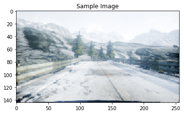
A phenomenon we can immediately observe is that only a small portion of the image is of interest. For example, we should be able to decide how to drive a car by focusing on the ROI in the red part of the figure below

sample_image_roi = sample_image.copy()

fillcolor=(255,0,0)
draw = ImageDraw.Draw(sample_image_roi)
points = [(1,76), (1,135), (255,135), (255,76)]
for i in range(0, len(points), 1):
    draw.line([points[i], points[(i+1)%len(points)]], fill=fillcolor, width=3)
del draw

plt.title('Image with sample ROI')
plt.imshow(sample_image_roi)
plt.show()

Extracting this ROI will reduce the training time and the amount of data required for the training model. It also prevents the model from being confused by focusing on irrelevant features in the environment, such as mountains, trees, etc.

Another observation we can make is that the data set shows the tolerance of vertical flip. In other words, we get a valid data point if we flip the image around the Y axis, if we also flip the symbol of the steering angle. This is very important because it effectively doubles the number of data points we have.

In addition, the trained model should remain unchanged to the changes of lighting conditions, so we can generate additional data points by globally scaling the brightness of the image.

Thinking exercise 0.1:
Once you have completed this tutorial, as an exercise, you should try to modify it using the provided dataset without using one or more of the three changes described above, leaving everything else unchanged. Will you experience very different results?

Thinking exercise 0.2:
We mentioned in Readme that end-to-end deep learning eliminates the need for manual feature engineering before inputting data into the learning algorithm. Would you consider these preprocessing changes to the dataset as engineering properties? Why or why not?

Now, let's aggregate all non image data into one data frame for more insights.

full_path_raw_folders = [os.path.join(RAW_DATA_DIR, f) for f in DATA_FOLDERS]

dataframes = []
for folder in full_path_raw_folders:
    current_dataframe = pd.read_csv(os.path.join(folder, 'airsim_rec.txt'), sep='\t')
    current_dataframe['Folder'] = folder
    dataframes.append(current_dataframe)
    
dataset = pd.concat(dataframes, axis=0)

print('Number of data points: {0}'.format(dataset.shape[0]))

dataset.head()

Number of data points: 46738

	Timestamp	Speed (kmph)	Throttle	Steering	Brake	Gear	ImageName	Folder
0	93683464	0	0.0	0.000000	0.0	N	img_0.png	../../AirSim/EndToEndLearningRawData/data_raw/...
1	93689595	0	0.0	0.000000	0.0	N	img_1.png	../../AirSim/EndToEndLearningRawData/data_raw/...
2	93689624	0	0.0	-0.035522	0.0	N	img_2.png	../../AirSim/EndToEndLearningRawData/data_raw/...
3	93689624	0	0.0	-0.035522	0.0	N	img_3.png	../../AirSim/EndToEndLearningRawData/data_raw/...
4	93689624	0	0.0	-0.035522	0.0	N	img_4.png	../../AirSim/EndToEndLearningRawData/data_raw/...

Now let's deal with the naming of dataset folders. You will notice that there are two types of folders in our dataset - 'normal' and 'swerve'. These names refer to two different driving strategies. Let's take a look at the differences between the two driving styles. First, we will plot part of the data points from each driving style.

min_index = 100
max_index = 1100
steering_angles_normal_1 = dataset[dataset['Folder'].apply(lambda v: 'normal_1' in v)]['Steering'][min_index:max_index]
steering_angles_swerve_1 = dataset[dataset['Folder'].apply(lambda v: 'swerve_1' in v)]['Steering'][min_index:max_index]

plot_index = [i for i in range(min_index, max_index, 1)]

fig = plt.figure(figsize=FIGURE_SIZE)
ax1 = fig.add_subplot(111)

ax1.scatter(plot_index, steering_angles_normal_1, c='b', marker='o', label='normal_1')
ax1.scatter(plot_index, steering_angles_swerve_1, c='r', marker='o', label='swerve_1')
plt.legend(loc='upper left');
plt.title('Steering Angles for normal_1 and swerve_1 runs')
plt.xlabel('Time')
plt.ylabel('Steering Angle')
plt.show()

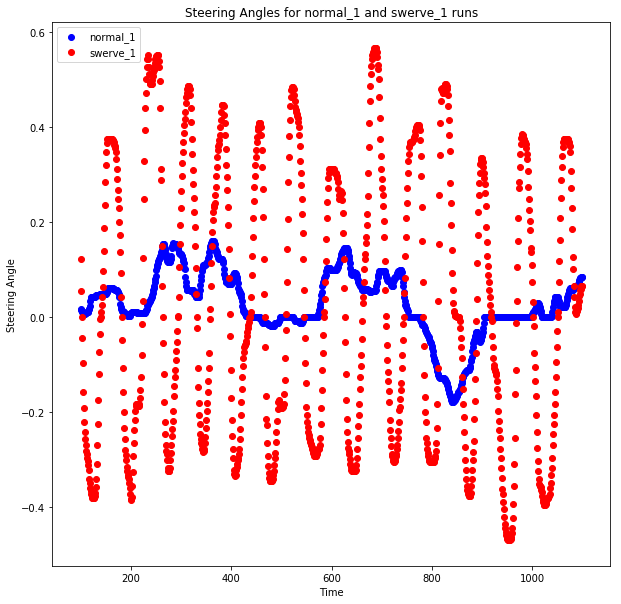
Here we can see the obvious difference between the two driving strategies. The blue dot shows the normal driving strategy. As you expected, it makes your steering angle more or less close to zero, which makes your car go straight on most of the road.

The sharp turn driving strategy makes the vehicle almost swing left and right on the road. This shows a very important thing to remember when training the end-to-end deep learning model. Because we didn't do any feature engineering, our model almost completely depends on the data set to provide all the necessary information it needs in the recall process. Therefore, in order to consider any sharp turn that the model may encounter and give it the ability to correct itself when it begins to deviate from the road, we need to provide it with enough examples during training. Therefore, we created these additional data sets to focus on these scenarios. Once you have completed the tutorial, you can try to rerun everything using only the "normal" dataset and see your car on the road for a long time.

• Thinking exercise 0.3
  What other data collection techniques do you think are needed in this steering angle prediction scenario? What about the general automatic driving?
  Now let's look at the number of data points in each category.

dataset['Is Swerve'] = dataset.apply(lambda r: 'swerve' in r['Folder'], axis=1)
grouped = dataset.groupby(by=['Is Swerve']).size().reset_index()
grouped.columns = ['Is Swerve', 'Count']

def make_autopct(values):
    def my_autopct(percent):
        total = sum(values)
        val = int(round(percent*total/100.0))
        return '{0:.2f}%  ({1:d})'.format(percent,val)
    return my_autopct

pie_labels = ['Normal', 'Swerve']
fig, ax = plt.subplots(figsize=FIGURE_SIZE)
ax.pie(grouped['Count'], labels=pie_labels, autopct = make_autopct(grouped['Count']))
plt.title('Number of data points per driving strategy')
plt.show()

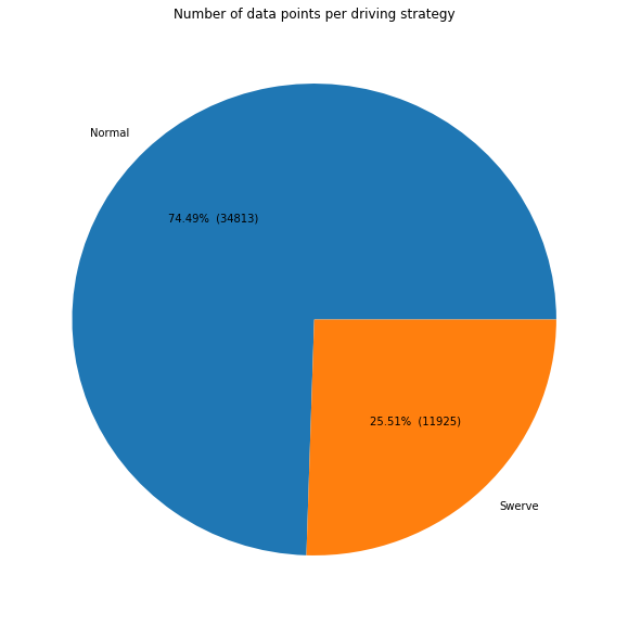
Therefore, about a quarter of the data points are collected through the steering driving strategy, and the rest are collected through the ordinary driving strategy. We also see that we have nearly 47000 data points to process. This is almost not enough data, so our network can't be too deep.

• Thinking exercise 0.4
  Like many things in the field of machine learning, the ideal proportion of data points in each category here is problem specific and can only be optimized by trial and error. Can you find a better one than ours?
  Let's look at the label distribution of these two strategies.

bins = np.arange(-1, 1.05, 0.05)
normal_labels = dataset[dataset['Is Swerve'] == False]['Steering']
swerve_labels = dataset[dataset['Is Swerve'] == True]['Steering']

def steering_histogram(hist_labels, title, color):
    plt.figure(figsize=FIGURE_SIZE)
    # It needs to be modified here: as_ Modify matrix() to values
    n, b, p = plt.hist(hist_labels.values, bins, normed=1, facecolor=color)
    plt.xlabel('Steering Angle')
    plt.ylabel('Normalized Frequency')
    plt.title(title)
    plt.show()

steering_histogram(normal_labels, 'Normal label distribution', 'g')
steering_histogram(swerve_labels, 'Swerve label distribution', 'r')

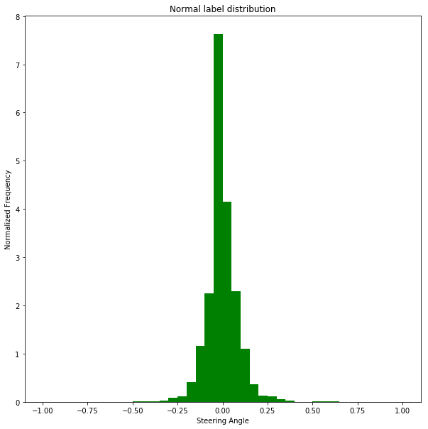
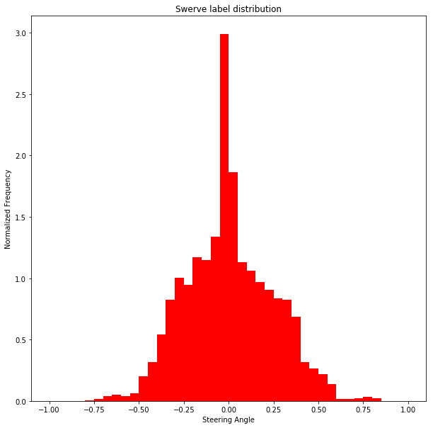
We can make some observations on the data in these charts:

• During normal driving, the steering wheel angle is almost always zero. There is a serious imbalance. If this part of data is not down sampled, the model will always predict zero and the car will not be able to turn.
• **When using the steering strategy to drive a car, we get some examples of sharp turns that do not appear in the conventional strategy data set** This confirms the reason why we collect the above data
  At this point, we need to merge the original data into a compressed data file suitable for training. Here, we will use h5 file, because this format is very suitable for supporting large data sets without reading all the data into memory at one time. It also works seamlessly with Keras.
  The code for generating data sets is simple, but long. When it terminates, the final dataset will have four parts:
• Image: numpy array containing image data
• previous_state: numpy array, containing the last known state of the car. This is a (steering, throttle, brake, speed) tuple
• label: numpy array, containing the steering angle we want to predict (normalized in the range of - 1... 1)
• metadata: numpy array, containing metadata about files (which folder they come from, etc.)
  Processing may take some time. We will also combine all data sets into one, and then split it into training / test / verification data sets.

train_eval_test_split = [0.7, 0.2, 0.1]
full_path_raw_folders = [os.path.join(RAW_DATA_DIR, f) for f in DATA_FOLDERS]
Cooking.cook(full_path_raw_folders, COOKED_DATA_DIR, train_eval_test_split)

Reading data from ../../AirSim/EndToEndLearningRawData/data_raw/normal_1...
Reading data from ../../AirSim/EndToEndLearningRawData/data_raw/normal_2...
Reading data from ../../AirSim/EndToEndLearningRawData/data_raw/normal_3...
Reading data from ../../AirSim/EndToEndLearningRawData/data_raw/normal_4...
Reading data from ../../AirSim/EndToEndLearningRawData/data_raw/normal_5...
Reading data from ../../AirSim/EndToEndLearningRawData/data_raw/normal_6...
Reading data from ../../AirSim/EndToEndLearningRawData/data_raw/swerve_1...
Reading data from ../../AirSim/EndToEndLearningRawData/data_raw/swerve_2...
Reading data from ../../AirSim/EndToEndLearningRawData/data_raw/swerve_3...
Processing ../../AirSim/EndToEndLearningRawData/data_cooked/train.h5...
Finished saving ../../AirSim/EndToEndLearningRawData/data_cooked/train.h5.
Processing ../../AirSim/EndToEndLearningRawData/data_cooked/eval.h5...
Finished saving ../../AirSim/EndToEndLearningRawData/data_cooked/eval.h5.
Processing ../../AirSim/EndToEndLearningRawData/data_cooked/test.h5...
Finished saving ../../AirSim/EndToEndLearningRawData/data_cooked/test.h5.

Now we are ready to start building the model. reach Next notebook Let's go.