Multiscale perception V3 method with efficient fine tuning
introduce
Every year, there are more than 230 people in the United States,000 The diagnosis of a person with breast cancer depends on whether the cancer has metastases. Metastasis detection is performed by pathologists examining large areas of biological tissue. This process is labor-intensive and error prone.
In today's project, our goal is to realize the multi-scale metastasis classification model proposed in the paper "detection of cancer metastasis on Gigapixel pathological images" arxiv: 1703.02442.
data set
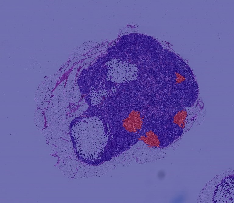
We used CAMELYON-16 Multi Giga Pixel data. 22 films with significant tumors were sampled from the main data set. Each film has a corresponding mask to mark the tumor area. We can achieve 9 magnification.
Each multi-scale image is superimposed on another image in a consistent coordinate system to allow users to access any image segment with any magnification.
We use OpenSlide C library and its Python binding to effectively access compressed files with the size of one billion pixels.

Data preparation
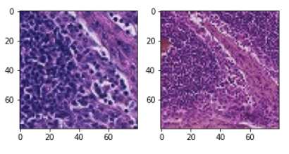
As the first step in generating marker training data, we use the sliding window method to slide at a higher zoom level and create marker images of fragments. We will use these images for training and testing later.
Using the method followed in this paper, we define a central window. If the center contains at least one pixel labeled as tumor, we mark the image as containing tumor cells.
The window size and center size are selected as 80 and 50, respectively. Finally, in order to make our training data multi-scale, we created a reduced version of the original image fragment of similar size. The reduced version is used to provide a macro level context for the classification model. We use a multi-scale method to generate data and use two different magnification to prepare the data set.
def generate_images(slide, slide_mask, level_1, level_2, window_size, center_size, stride):
  """
  The function generates training data at two different magifications.
  """

  tumor_image = read_slide(slide,
                         x=0,
                         y=0,
                         level=level_1,
                         width=tumor.level_dimensions[level_1][0],
                         height=tumor.level_dimensions[level_1][1])

  tumor_mask_image = read_slide(slide_mask,
                         x=0,
                         y=0,
                         level=level_1,
                         width=tumor.level_dimensions[level_1][0],
                         height=tumor.level_dimensions[level_1][1])

  tumor_mask_image = tumor_mask_image[:,:,0]
  patch_images = []
  patch_labels = []
  patch_center = []
  patch_coord  = []

  count = 0
  tumor_count = 0
  health_count = 1

  for i in range(window_size//2, slide.level_dimensions[level_1][1] - window_size - stride, stride):
    for j in range(window_size//2, slide.level_dimensions[level_1][0] - window_size - stride, stride):

      patch = tumor_image[i:i+window_size, j:j+window_size]
      tumor_mask_patch = tumor_mask_image[i:i+window_size, j:j+window_size]

      tissue_pixels = find_tissue_pixels(patch)
      tissue_pixels = list(tissue_pixels)
      percent_tissue = len(tissue_pixels) / float(patch.shape[0] * patch.shape[0]) * 100

      # If contains a tumor in the center
      if check_centre(tumor_mask_patch, center_size):
        patch_images.append(patch)
        patch_labels.append(1)
        patch_coord.append((j, i))
        patch_center.append((j+window_size//2, i+window_size//2))
        tumor_count += 1
        continue

      # If healthy keep only if the image patch contains more than 50% tissue
      # and sample to keep the memory size small

      if percent_tissue > 75:
        if (health_count < tumor_count) or (np.random.uniform() > (1 - tumor_count/(health_count+tumor_count))):
          patch_images.append(patch)
          patch_labels.append(0)
          patch_coord.append((j, i))
          patch_center.append((j+window_size//2, i+window_size//2))
          health_count += 1

      count += 1

  tumor_ids = [id for id in range(len(patch_labels)) if int(patch_labels[id]) == 1]
  normal_ids = [id for id in range(len(patch_labels)) if int(patch_labels[id]) == 0]

  # Randomly Shuffle the images
  np.random.shuffle(tumor_ids)
  np.random.shuffle(normal_ids)
  total_ids = tumor_ids + normal_ids
  np.random.shuffle(total_ids)

  patch_images = [patch_images[idx] for idx in total_ids]
  patch_labels = [patch_labels[idx] for idx in total_ids]
  patch_center = [patch_center[idx] for idx in total_ids]
  patch_coord = [patch_coord[idx] for idx in total_ids]
  tumor_image = read_slide(slide,
                         x=0,
                         y=0,
                         level=level_2,
                         width=tumor.level_dimensions[level_2][0],
                         height=tumor.level_dimensions[level_2][1])
  patch_images_2 = []
  for center in patch_center:
      patch = tumor_image[center[1]//2-window_size//2:center[1]//2+window_size//2, center[0]//2-window_size//2:center[0]//2+window_size//2]
      assert patch.shape == (window_size, window_size, 3)
      patch_images_2.append(patch)
  return patch_images, patch_images_2, patch_labels, patch_coord
Data augmentation
We use various data enhancement techniques to supplement our training data and make our model more robust.
Orthogonal rotation and flip
We introduce orthogonal augmentation to introduce rotation invariance because slides can be checked in these directions
- Random orthogonal rotation
- Random horizontal and vertical flip
Color perturbation
In order to make our model robust to illumination and color intensity, we perturb the color as follows.
- The maximum brightness is 64 / 255
- Saturation, max. 0. twenty-five
- The maximum increment of hue is 0.04
- The maximum value is 0. seventy-five
#This function applies random brightness, saturation, hue, and constrast to the training images
# The Max Delta Values have been taken directly from the paper
def data_augmentation(img):
    img = tf.image.random_brightness(img, 64.0/255)
    img = tf.image.random_saturation(img, 0.75, 1)
    img = tf.image.random_hue(img, 0.04)
    img = tf.image.random_contrast(img, 0.50, 1)
    return img

#This function applies orthogonal rotation transformations to the training data
def orthogonal_rotations(img):
    return np.rot90(img, np.random.choice([-1, 0, 1, 2]))

# The function maps the pixel values between (-1, 1)
def rescale(image):
    image = image / 255.0
    image = (image - 0.5) * 2
    return image

def preprocess(image):
    image = orthogonal_rotations(image)
    image = data_augmentation(image)
    image = rescale(image)
    return image
Implementation method
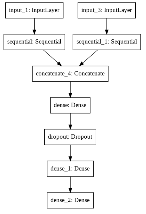
We use the multi tower perception V3 model to classify multi-scale images. We only fine tune the top layer, because these layers learn higher-level features. By fine tuning these layers based on our data set, the results can be greatly improved.
Architecture used: inception V3 (multi-scale) fine tuned for > 150 layers
Initial weight: Image Net
Loss function: binary cross entropy loss
Magnification: Level 2 and 3
result
We finally tested our model on a new tumor section. After preprocessing the tumor slices and making predictions, we created a heat map using the model output.
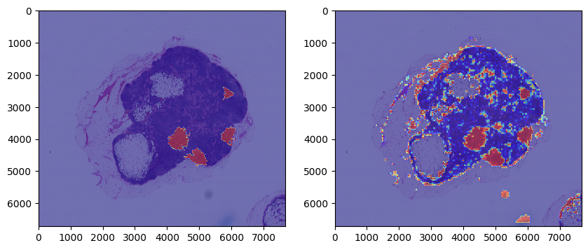
- AUC: 0.97659
- Threshold: 0.48429
- Sensitivity: 0.97478
- Specificity: 0.95004
- Recall: 0.97277
- Precision: 0.22275
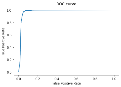
We saw that all tumor areas were correctly identified.
We can have a high recall rate (which is important in medical prognosis)
Transfer learning with fine tuning can effectively produce good results under the condition of low computational intensity
This model does not seem to predict the boundary accurately.
Future improvements
Use higher magnification images to get better GPU and larger RAM. By calculating the prediction of each possible sliding direction, the prediction average is used to improve the accuracy and introduce rotation invariance. Better foreground and background separation techniques are used to improve the performance of the boundary.
Author: Smarth Gupta
Deep hub translation group