1, Introduction to methylation chip
A chip includes 12 array s, that is, a chip can make 12 samples, and a machine can run 8 chips, that is, a total of 96 samples. Each sample can measure the methylation information of more than 450000 CpG sites (about 1% of all people, but covers most CpG islands and promoter regions). The chip itself contains some control probes for quality control.
Chip comment information:
#View 450k chip comment information
library(IlluminaHumanMethylation450kmanifest)
show(IlluminaHumanMethylation450kmanifest)

#View 850k chip information and use another R package
library(IlluminaHumanMethylationEPICkmanifest)
There is a specific function getManifest() in the minfi package to view the annotation information of the chip corresponding to the specified object
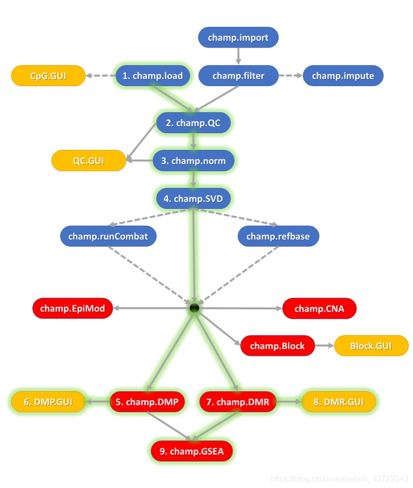
2, Introduction to camp package
Camp can be used to process 450k and EPIC data. Functions such as quality control, data standardization, DMR identification and CNA identification are integrated in the package to form a pipeline for the processing of methylation data.
If the parameters in your whole process are set to the default value, you only need to run the function: champ.process(directory = testDir), and the parameter directory is the file directory where the methylation raw data. IDAT is located.
Of course, each function in camp can also be run separately with custom parameters.
3, Specific processing flow
(1) Data preparation
The camp package needs not only the. idat original file, but also a pd(phenotype) file named sample to read data_ Sheet.csv (of course, the name sample_sheet is not important, but it is a * *. CSV file * *). The specific information is as follows:
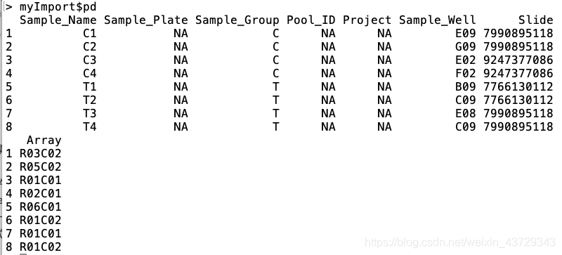
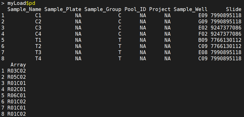
The more important attribute column is Sample_Name,Sample_Group,Slide(Sentrix_ID),Array(Sentrix_position)
Array (Sentrix_position): there are up to 12 samples on a methylation chip, and each sample is based on sentrix_ Position identification;
Slide (Sentrix_ID): when the number of samples is greater than 12, another chip is necessary. Sentrix is used for each chip_ ID identification;
minfi is through Sentrix_ID and Sentrix_position these two fields to find the original data of the sample
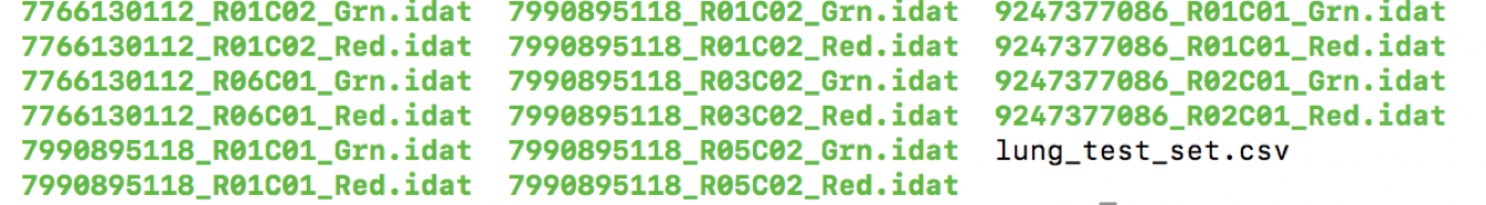
You need to create a sample according to the sample information_ Sheet.csv, how to build? Sentrix_ID and Sentrix_Position comes from the IDAT file name.
Note: the data downloaded by GEO is named by the submitter, so it is difficult to build the csv file. TCGA downloads the data, and the file name contains the required information. You can build the csv file
1. Use the data in the ChAMPdata package
library(ChAMP)
testdir<-system.file("extdata",package="ChAMPdata")
Go to the above path to view the data:
testDir[1]="/public/workspace/shaojf/anaconda3/lib/R/library/ChAMPdata/extdata"
It contains 8 samples, 4 tumor samples and 4 control samples
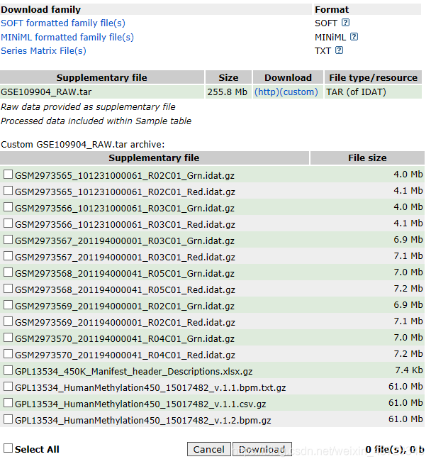
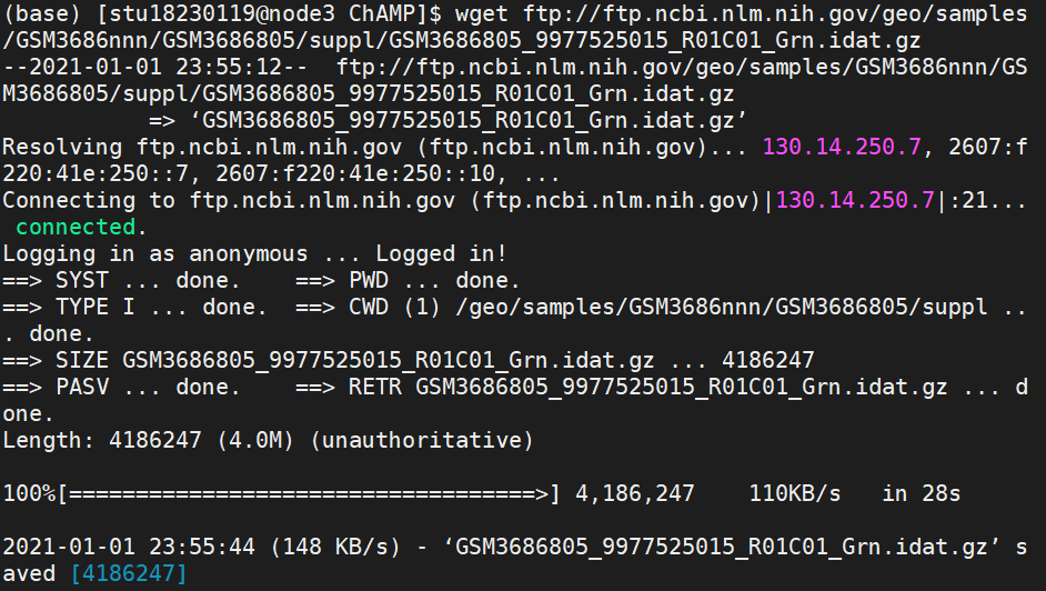
2. Database download. Take GEO as an example to illustrate data preparation
(2) Data reading and filtering champ.load
myLoad <-champ.load(testDir,arraytype="450K")
#The chip type can be set to "EPIC" to load the data of 850K chip
See champ.import() and champ.filter() for champ.load() parameters. champ.load() uses minfi package to read data
champ.load()==champ.import()+champ.filter()
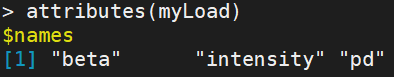
Return a list containing three elements: "beta", "intensity", "pd"
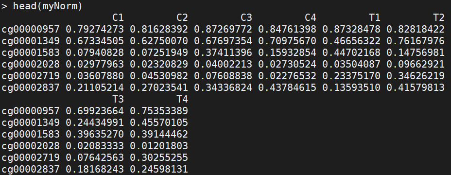
beta is a matrix with columns representing samples and rows representing probes
pd records the sample information, that is, the sample written by yourself_ Sheet.csv file, important attribute columns "Slide", "Array"
There are 6 kinds of data filtering after reading data:
① filterDetP, detPcut: probes < 0.01 are filtered out by default, and detPcut is used to modify the threshold
② filterBeads, beadCutoff: the probe hybridizes with the DNA sequence. beadcounts is the number of reads combined with the probe. If the combination is less, it is considered that the probe signal is unreliable. In actual processing, the default is that if the probe is in 5% of the samples and the beadcount is less than 3, the probe will be filtered out. Use beadCutoff to modify the threshold
③ filterNoCG: filter probes at non CpG sites. For methylated C, there are methylated C such as CpG\CHG\CHH. If you do not want to filter these probes, you can set filterNoCG=FALSE
④ filterSNPs: filter the probe of CpG site near SNP. The CPG site near SNP site is unstable. Set filterSNPs=FALSE to not filter
⑤ filterMultiHit: filter nonspecific probes. Nordlund and other researchers use bwa to compare the probe sequence with the genome. If the only comparison indicates that the probe has good specificity, remove the probes aligned to multiple positions on the genome according to the comparison results, and modify the parameter filterMultiHit=FALSE to not filter
⑥ filterXY: filter the probe on the sex chromosome. The difference CpG on the sex chromosome is inaccurate. It is impossible to explain whether the difference is caused by the experiment. If the gender is the same, you can not filter. Modify the parameter filterXY=FALSE and do not filter
(3) Visual view of quality control champ.QC
champ.QC(beta = myLoad$beta,
		 #---Generated β matrix
		 pheno=myLoad$pd$Sample_Group,
		 #---Sample classification information
		 mdsPlot=TRUE,
		 densityPlot=TRUE,
		 dendrogram=TRUE,
         PDFplot=TRUE,Rplot=TRUE,
		 Feature.sel="None",
		 #---Calculation method used when drawing dendrogram
		 resultsDir="./CHAMP_QCimages/")
QC.GUI()
(4) Data standardization champ.norm
The correction of the probe is to eliminate the error caused by the technical difference between the two types of probes
myNorm<-champ.norm(beta=myLoad$beta,rgSet=myLoad$rgSet,mset=myLoad$mset,
			resultsDir=".CHAMP_Normalization/",
			method="BMIQ",
			plotBMIQ=FALSE,
			arraytype="450K",
			cores=3)
(5) Batch effect
1. Check whether there is batch effect champ.SVD
champ.SVD(beta = myNorm,
		   rgSet=NULL,
		   pd=myLoad$pd,
		   RGEffect=FALSE,
		   #---If Green and Red color control probes would be calculated
          PDFplot=TRUE,Rplot=TRUE,
		  resultsDir="./CHAMP_SVDimages/")
Generate 2 images: Singular Value Decomposition Analysis (SVD); Scree Plot
①Singular Value Decomposition Analysis (SVD)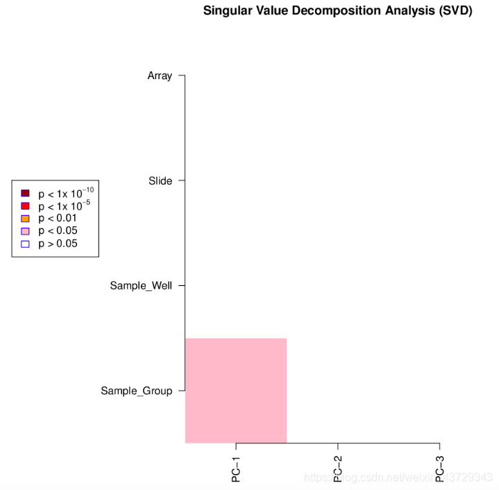
The darker the color, the smaller the p-value, and the more significant the variation, indicating that the greater the variation component
It can be seen from the image that the variation mainly comes from between samples (control group and tumor group), that is, the biological factors we pay attention to, but the variation is not significant. The filtered data is clear and suitable for subsequent analysis.
If significant p-value s are found in array or slide, it is necessary to check the experimental design and use other normalization methods for subsequent batch effect correction
②scree plot:
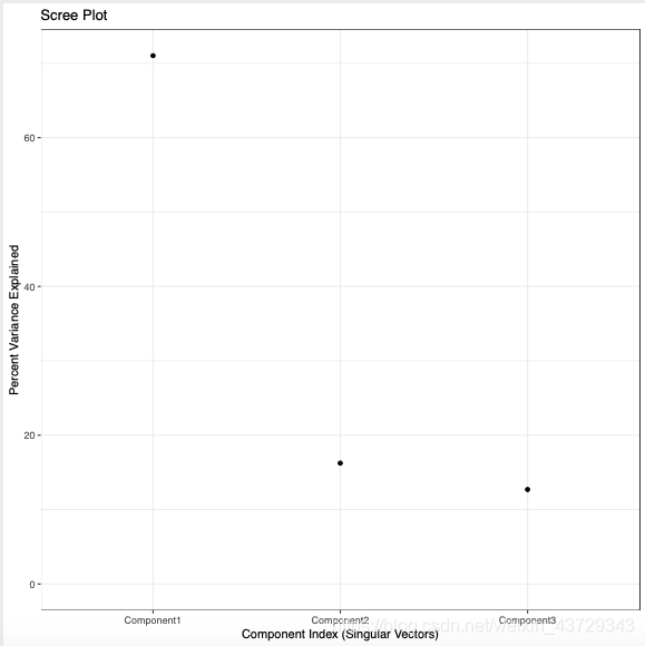
The percentage of the variation that can be explained by each principal component in the total variation
2. Correct batch effect champ.runCombat
mycombat <- champ.runCombat(beta=myNorm,
				pd=myLoad$pd,
                variablename="Sample_Group",
				#For the covariates to be corrected, refer to the ComBat function of the sva package
				batchname=c("Slide"),
				#Batch from pd file
                logitTrans=TRUE)
				#Whether the beta is logit transformed is set to T when using the original beta for correction and F when using the M value for calculation
If ComBat is directly corrected with beta value, the output value may not be between 0-1, so a logit will be converted to M-value before calculation;
If M value is used for correction, conversion is not necessary, so set logitTrans=F
(6) Methylation analysis
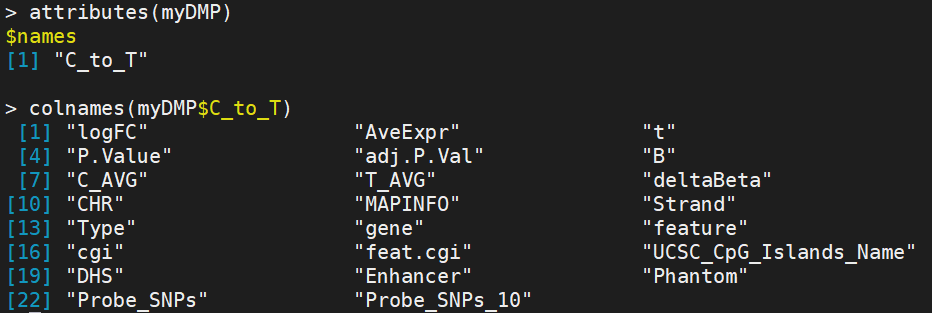
1.champ.DMP
myDMP <- champ.DMP(beta = myNorm,
	  				pheno = myLoad$pd$Sample_Group,
      				compare.group = NULL,
	 	 			#When group > 2, set this parameter as a list, where each element is two samples_ Group, and then specify the group to be compared. Otherwise, every two groups will be compared
     				adjPVal = 0.05,
      				#Set p-value test level
	  				adjust.method = "BH",
	  				#p-value correction, using the method reference function p.adjust()
      				arraytype = "450K")
#DMP is calculated directly by probe comparison based on category group

# Visual view of distribution
DMP.GUI(DMP=myDMP[[1]],beta=myNorm,pheno=myLoad$pd$Sample_Group)
#shiny package is required to use GUI
2.champ.DMR
myDMR<-champ.DMR(beta=myNorm,
          pheno=myLoad$pd$Sample_Group,
          compare.group=NULL,
          arraytype="450K",
          method = "Bumphunter",
          minProbes=7,
          #---DMR contains many CpG sites, and each site corresponds to a probe. minProbes sets the minimum number of probes contained in each DMR
          adjPvalDmr=0.05,
          #---The p-value of DMR is calculated by Stouffler's method, and then corrected to obtain adjPvalDmr
          cores=3,
          ## following parameters are specifically for Bumphunter method.
          maxGap=300,
          cutoff=NULL,
          pickCutoff=TRUE,
          smooth=TRUE,
          smoothFunction=loessByCluster,
          useWeights=FALSE,
          permutations=NULL,
          B=250,
          nullMethod="bootstrap",
          ## following parameters are specifically for probe ProbeLasso method.
          meanLassoRadius=375,
          minDmrSep=1000,
          minDmrSize=50,
          adjPvalProbe=0.05,
          Rplot=T,
          PDFplot=T,
          resultsDir="./CHAMP_ProbeLasso/",
          ## following parameters are specifically for DMRcate method.
          rmSNPCH=T,
          fdr=0.05,
          dist=2,
          mafcut=0.05,
          lambda=1000,
          C=2)

# Visual view of distribution
DMR.GUI(DMR=myDMR)