deep learning "hello world“( [deep learning practice 1]: handwritten numeral recognition based on Keras (very detailed, open source code) )It has been updated. If you can recognize handwritten digits, it means that one foot has stepped into the door of deep learning!

  today, the blogger brings the second practical content: cifar10 image classification based on Keras. It's all dry goods. A complete code is attached at the end of the article!

1, Preparatory work

Devices \ Libraries	Model \ version
Graphics card	GTX1650
Driver version	457.49
Tensorflow GPU version	2.4.0
keras version	2.4.3
Python version	3.7.3

2, Download cifar10 dataset

Keras has integrated the cifar10 dataset, which can be downloaded and used directly through the API.

2.1 import required libraries and modules

from keras.datasets import cifar10
import matplotlib.pyplot as plt

2.2 downloading data sets

# x_train_original and y_train_original represent the images and labels of the training set, and x_test_original and y_test_original represent the images and labels of the test set
(x_train_original, y_train_original), (x_test_original, y_test_original) = mnist.load_data()

The downloaded datasets will be stored in the datasets folder in. keras under the user of Disk C:

C:\Users\Lenovo\.keras\datasets

3, Data set preprocessing

3.1 image label visualization

   we need to know what the images of the cifar10 dataset represent respectively. First, we decompress the dataset compression package, and you can see that there is a batches.meta file, which contains some information of the image; data_batch_1~5 represents the batch of the training set; test_batch represents the batch of the test set.

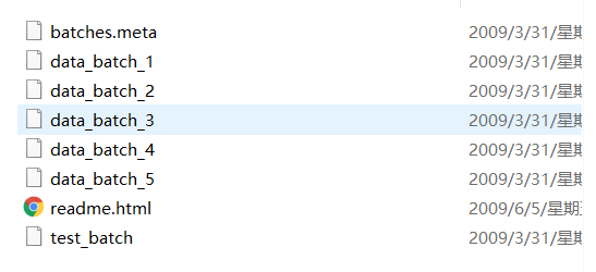
We define the following function to visualize this information:

def load_file(filename):
    with open(filename, 'rb') as datasets:
        data = pickle.load(datasets)
    return data

Call this function:

data = load_file(r'C:\Users\Lenovo\.keras\datasets\cifar-10-batches-py\batches.meta')

We print data information:

print(data.keys())  # Print key name
print(data.values())  # Print key value

The output result is:

dict_keys(['num_cases_per_batch', 'label_names', 'num_vis'])
dict_values([10000, ['airplane', 'automobile', 'bird', 'cat', 'deer', 'dog', 'frog', 'horse', 'ship', 'truck'], 3072])

From the output results, we can get several information:

• Key name: the number of images in the training set of each Batch, the label name, and the number of pixels in a single image
• Key value: each Batch of the training set contains 10000 images. The images have 10 labels, namely, 'airplane', 'automobile', 'bird', 'cat', 'der', 'dog', 'frog', 'horse', 'ship', 'truck'. The number of pixels in a single image is 3072, which is composed of 32 × thirty-two × 3, because the size of the image is (32 × thirty-two × 3) , we'll talk about it later.

3.2 other treatment

The next preprocessing steps include:

• Image visualization (single image visualization, multiple image visualization)
• Allocate validation set (in terms of data set volume, it is recommended to extract half of the test set as the validation set)
• Image data preprocessing (type conversion: uint8 type to float32 type; image normalization)
• Image label preprocessing (the coding mode is changed to single heat coding)

See the program utils.py for details

# -*- coding = utf-8 -*-
# @time:2021/11/28/0028 21:42 PM
# Author: Michelangelo
# @File:utils.py
# @Software:PyCharm

# Program introduction
"""
utils.py Contains a pair of cifar10 All preprocessing and visualization processes of data set
"""


"""
Library import
"""
from keras.datasets import cifar10
import matplotlib.pyplot as plt
import pickle
from keras.utils import np_utils


"""
Data set download and loading (using KerasAPI)
"""
# x_train_original and y_train_original represent the images and labels of the training set, and x_test_original and y_test_original represent the images and labels of the test set
(x_train_original, y_train_original), (x_test_original, y_test_original) = cifar10.load_data()


"""
Print dataset information
"""
# File processing function (visual image original label), and the location of calling this function is in the subsequent function load_data()
def load_file(filename):
    with open(filename, 'rb') as datasets:
        data = pickle.load(datasets)
    return data


"""
Dataset image visualization (the part that calls these two functions is described later load_data()Medium)
"""
# Single image visualization (select an image visualization by index)
# When mode=0, select the data visualization of the original training set; when mode is other, select the data visualization of the original test set
def mnist_visualize_single(mode, idx):
    if mode == 0:
        plt.imshow(x_train_original[idx], cmap=plt.get_cmap('gray'))        # Display function
        title = 'label=' + str(y_train_original[idx])                       # Tag name (here is the original coded tag, i.e. 0 ~ 9)
        plt.title(title)
        plt.xticks([])  # The x-axis is not displayed
        plt.yticks([])  # The y-axis is not displayed
        plt.show()      # image display
    else:
        plt.imshow(x_test_original[idx], cmap=plt.get_cmap('gray'))
        title = 'label=' + str(y_test_original[idx])
        plt.title(title)
        plt.xticks([])  # The x-axis is not displayed
        plt.yticks([])  # The y-axis is not displayed
        plt.show()


# Multi image visualization
# The start and end parameters of the function indicate that the visualization starts from start and ends from end. For example, start=4 and end=8 indicate images with visualization indexes of 4, 5, 6 and 7 (Note: start with strat and end-1)
# The length and width parameters of the function represent the display of the image in the drawing box. For example, length=3 and width=3 represent drawing a 3 × 3 (9 in total), which is used to place visual images
def mnist_visualize_multiple(mode, start, end, length, width):
    if mode == 0:
        for i in range(start, end):
            plt.subplot(length, width, 1 + i)
            plt.imshow(x_train_original[i], cmap=plt.get_cmap('gray'))
            title = 'label=' + str(y_train_original[i])
            plt.title(title)
            plt.xticks([])
            plt.yticks([])
        plt.show()
    else:
        for i in range(start, end):
            plt.subplot(length, width, 1 + i)
            plt.imshow(x_test_original[i], cmap=plt.get_cmap('gray'))
            title = 'label=' + str(y_test_original[i])
            plt.title(title)
            plt.xticks([])
            plt.yticks([])
        plt.show()


"""
Assign validation sets and visualize the number of parts
"""
def val_set_alloc():
    # Raw dataset data volume
    print('Size of the original training set image:', x_train_original.shape)
    print('Size of the original training set label:', y_train_original.shape)
    print('Size of the original test set image:', x_test_original.shape)
    print('Size of the original test set label:', y_test_original.shape)
    print('===============================')

    # Verification set allocation (extracted from the test set because the training set has insufficient data)
    x_val = x_test_original[:5000]
    y_val = y_test_original[:5000]
    x_test = x_test_original[5000:]
    y_test = y_test_original[5000:]
    x_train = x_train_original
    y_train = y_train_original

    # Print the data volume of each part after verification set allocation
    print('Size of training set image:', x_train.shape)
    print('Size of training set label:', y_train.shape)
    print('Verify the size of the set image:', x_val.shape)
    print('Verify the size of the set label:', y_val.shape)
    print('Size of test set image:', x_test.shape)
    print('Size of test set label:', y_test.shape)
    print('===============================')

    return x_train, y_train, x_val, y_val, x_test, y_test


"""
Image data and label data preprocessing
"""
def data_process(x_train, y_train, x_val, y_val, x_test, y_test):

    # Here, the data is transformed from unint type to float32 type to improve the training accuracy.
    x_train = x_train.astype('float32')
    x_val = x_val.astype('float32')
    x_test = x_test.astype('float32')

    # The pixel gray value of the original image is 0-255. In order to improve the training accuracy of the model, the value is usually normalized and mapped to 0-1.
    x_train = x_train / 255
    x_val = x_val / 255
    x_test = x_test / 255

    # There are 10 categories of image tags, i.e. 0-9, which are transformed into one hot vector
    y_train = np_utils.to_categorical(y_train)
    y_val = np_utils.to_categorical(y_val)
    y_test = np_utils.to_categorical(y_test)

    return x_train, y_train, x_val, y_val, x_test, y_test


"""
Load data (that is, all functions defined above are integrated through this function to output the final image data and labels)
"""
def load_data():

    # Print dataset information
    data = load_file(r'C:\Users\Lenovo\.keras\datasets\cifar-10-batches-py\batches.meta')
    print(data.keys())              # Print key name
    print(data.values())            # Print key value

    # Visual image data
    mnist_visualize_single(mode=0, idx=0)
    mnist_visualize_multiple(mode=0, start=0, end=9, length=3, width=3)

    # Validation set allocation
    x_train, y_train, x_val, y_val, x_test, y_test = val_set_alloc()

    # Data preprocessing (image data, label data)
    x_train, y_train, x_val, y_val, x_test, y_test = data_process(x_train, y_train, x_val, y_val, x_test, y_test)

    return x_train, y_train, x_val, y_val, x_test, y_test

if __name__ == '__main__':
    load_data()

The program output result is:

dict_keys(['num_cases_per_batch', 'label_names', 'num_vis'])
dict_values([10000, ['airplane', 'automobile', 'bird', 'cat', 'deer', 'dog', 'frog', 'horse', 'ship', 'truck'], 3072])
Size of the original training set image: (50000, 32, 32, 3)
Size of the original training set label: (50000, 1)
Size of the original test set image: (10000, 32, 32, 3)
Size of the original test set label: (10000, 1)
===============================
Size of training set image: (50000, 32, 32, 3)
Size of training set label: (50000, 1)
Verify the size of the set image: (5000, 32, 32, 3)
Verify the size of the set label: (5000, 1)
Size of test set image: (5000, 32, 32, 3)
Size of test set label: (5000, 1)
===============================

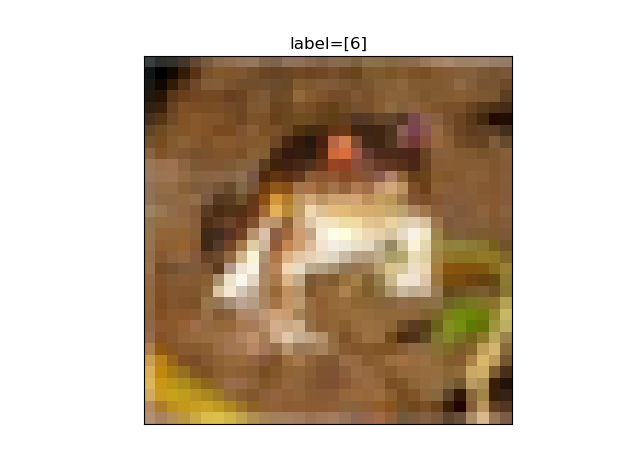
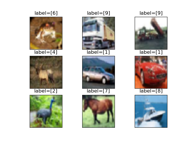
4, Network construction

4.1 construction of conventional convolutional neural network

We build a program file called net.py!
First, we import library functions:

import matplotlib.pyplot as plt
from tensorflow.keras.models import Sequential
from keras.models import Model
from tensorflow.keras.layers import Conv2D, MaxPooling2D, Flatten, Dense, BatchNormalization, Input, add, Dropout
from keras.utils.vis_utils import plot_model
import tensorflow as tf
import os

Now start defining regular CNN,
The selection of activation function and why to use single heat coding have been explained in the program.

"""
routine CNN Model
"""
# Description of activation function selection:
# (1) The convolution layer selects "relu" activation function: in a sense, the relu activation function is the best activation function, which is applicable to many scenes. It performs very well on the convolution layer because the convergence speed of the relu activation function is very fast,
# The gradient will not be saturated, which alleviates the problem of gradient disappearance, and the calculation speed is faster. While the sigmoid activation function and tanh activation function are gradually flat in the positive interval, and there is almost no gradient change,
# This will cause the network gradient weight can not be updated, resulting in the network can not be trained, the neural network can not enter the gradient minimum point, and there is no network optimal value.
#(2) The last layer of Dense selects the "softmax" activation function: the selection of the activation function here is related to the encoding method of the dataset label. Specifically, the encoding method of the dataset label is unique heat encoding, which represents one
# For a sequence with a length of 10, only 0 and 1 represent and only one 1, and the others are 0. In addition, the position of 1 in the sequence = the value of the original label.
# For example: if the label of an image is 4, the unique thermal coding result is 0 0 0 0 1 0 0 0 0 0 0 0 0 0 0 0 0 0 0 0 0 0 0 0 0 0 0 0 0 0 0 0 0 0 0 0 0 0 0 0 0 0 0 0 0 0 0 0 0 0 0 0 0 0 0 0 0 0 0 0 0 0 0 0 0 0 0 0 0 0 0.
# The output of softmax activation function is the probability value, that is, no matter how many categories the data set has, the sum of the prediction results of all categories is 1, then the position where the highest probability category in these categories appears with the 1 of the unique heat code, if
# The same indicates that the network prediction is correct, then the network can continue training according to the gradient change, on the contrary, change the training direction.
# (3) To sum up: single hot coding and softmax are often used together.
def conventional_model():
    model = Sequential()        # Using sequential model

    model.add(Conv2D(filters=32, kernel_size=(3, 3), padding='same', activation='relu', input_shape=(32, 32, 3)))   # Add volume layer
    model.add(BatchNormalization())             # Adding a BN layer prevents overfitting

    model.add(Conv2D(filters=32, kernel_size=(3, 3), padding='same', activation='relu', input_shape=(32, 32, 3)))
    model.add(BatchNormalization())

    model.add(Conv2D(filters=64, kernel_size=(3, 3), activation='relu'))
    model.add(BatchNormalization())

    model.add(MaxPooling2D(pool_size=(2, 2), strides=(2, 2)))       # Add maximum pooling layer: downsampling, removing redundant information, feature compression, reducing computation, simplifying network complexity and increasing nonlinearity
    model.add(Flatten())                            # Add a tile layer to expand all the neurons of the feature map for the subsequent full connection layer
    model.add(Dense(256, activation='relu'))        # Add a full connection layer to start feature integration and image classification
    model.add(Dropout(0.5))                         # In order to prevent overfitting caused by too many parameters in the whole connection layer, randomly inactivated neurons in this layer are added
    model.add(Dense(10, activation='softmax'))      # The last layer is used as a classifier to output 10 neurons

    print(model.summary())                          # Print model

    # Model structure diagram output
    plot_model(model, to_file='conventional_model.png', show_shapes=True, show_layer_names=True, rankdir='TB')
    plt.figure(figsize=(10, 10))
    img = plt.imread('conventional_model.png')
    plt.imshow(img)
    plt.axis('off')
    plt.show()

    return model


if __name__ == '__main__':
    conventional_model()

The model output information is:

Model: "sequential"
_________________________________________________________________
Layer (type)                 Output Shape              Param #   
=================================================================
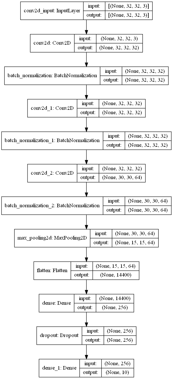
conv2d (Conv2D)              (None, 32, 32, 32)        896       
_________________________________________________________________
batch_normalization (BatchNo (None, 32, 32, 32)        128       
_________________________________________________________________
conv2d_1 (Conv2D)            (None, 32, 32, 32)        9248      
_________________________________________________________________
batch_normalization_1 (Batch (None, 32, 32, 32)        128       
_________________________________________________________________
conv2d_2 (Conv2D)            (None, 30, 30, 64)        18496     
_________________________________________________________________
batch_normalization_2 (Batch (None, 30, 30, 64)        256       
_________________________________________________________________
max_pooling2d (MaxPooling2D) (None, 15, 15, 64)        0         
_________________________________________________________________
flatten (Flatten)            (None, 14400)             0         
_________________________________________________________________
dense (Dense)                (None, 256)               3686656   
_________________________________________________________________
dropout (Dropout)            (None, 256)               0         
_________________________________________________________________
dense_1 (Dense)              (None, 10)                2570      
=================================================================
Total params: 3,718,378
Trainable params: 3,718,122
Non-trainable params: 256
_________________________________________________________________
None

The network structure diagram is:

4.2 construction of neural network with residual structure

Define network:

"""
With residual structure CNN Model
"""
def res_model():
    input_shape = Input(shape=(32, 32, 3))

    x1 = Conv2D(filters=32, kernel_size=(3, 3), padding='same', activation='relu')(input_shape)
    x1 = BatchNormalization()(x1)

    x2 = Conv2D(filters=32, kernel_size=(3, 3), padding='same', activation='relu')(x1)
    x2 = BatchNormalization()(x2)

    add1 = add([x1, x2])            # A jump connection is introduced for gradient updating to prevent gradient dispersion or explosion caused by too deep network

    x3 = Conv2D(filters=64, kernel_size=(3, 3), activation='relu')(add1)
    x3 = BatchNormalization()(x3)

    x4 = MaxPooling2D(pool_size=(2, 2), strides=(2, 2))(x3)
    x4 = Flatten()(x4)
    x4 = Dense(256, activation='relu')(x4)
    x4 = Dropout(0.5)(x4)
    output = Dense(10, activation='softmax')(x4)

    model = tf.keras.Model(input_shape, output)
    print(model.summary())
    validity = model(input_shape)

    plot_model(model, to_file='res_model.png', show_shapes=True, show_layer_names=True, rankdir='TB')
    plt.figure(figsize=(10, 10))
    img = plt.imread('res_model.png')
    plt.imshow(img)
    plt.axis('off')
    plt.show()

    return Model(input_shape, validity)


if __name__ == '__main__':
    res_model()

The model output information is:

Model: "model"
__________________________________________________________________________________________________
Layer (type)                    Output Shape         Param #     Connected to                     
==================================================================================================
input_1 (InputLayer)            [(None, 32, 32, 3)]  0                                            
__________________________________________________________________________________________________
conv2d (Conv2D)                 (None, 32, 32, 32)   896         input_1[0][0]                    
__________________________________________________________________________________________________
batch_normalization (BatchNorma (None, 32, 32, 32)   128         conv2d[0][0]                     
__________________________________________________________________________________________________
conv2d_1 (Conv2D)               (None, 32, 32, 32)   9248        batch_normalization[0][0]        
__________________________________________________________________________________________________
batch_normalization_1 (BatchNor (None, 32, 32, 32)   128         conv2d_1[0][0]                   
__________________________________________________________________________________________________
add (Add)                       (None, 32, 32, 32)   0           batch_normalization[0][0]        
                                                                 batch_normalization_1[0][0]      
__________________________________________________________________________________________________
conv2d_2 (Conv2D)               (None, 30, 30, 64)   18496       add[0][0]                        
__________________________________________________________________________________________________
batch_normalization_2 (BatchNor (None, 30, 30, 64)   256         conv2d_2[0][0]                   
__________________________________________________________________________________________________
max_pooling2d (MaxPooling2D)    (None, 15, 15, 64)   0           batch_normalization_2[0][0]      
__________________________________________________________________________________________________
flatten (Flatten)               (None, 14400)        0           max_pooling2d[0][0]              
__________________________________________________________________________________________________
dense (Dense)                   (None, 256)          3686656     flatten[0][0]                    
__________________________________________________________________________________________________
dropout (Dropout)               (None, 256)          0           dense[0][0]                      
__________________________________________________________________________________________________
dense_1 (Dense)                 (None, 10)           2570        dropout[0][0]                    
==================================================================================================
Total params: 3,718,378
Trainable params: 3,718,122
Non-trainable params: 256
__________________________________________________________________________________________________
None

The model structure diagram is:

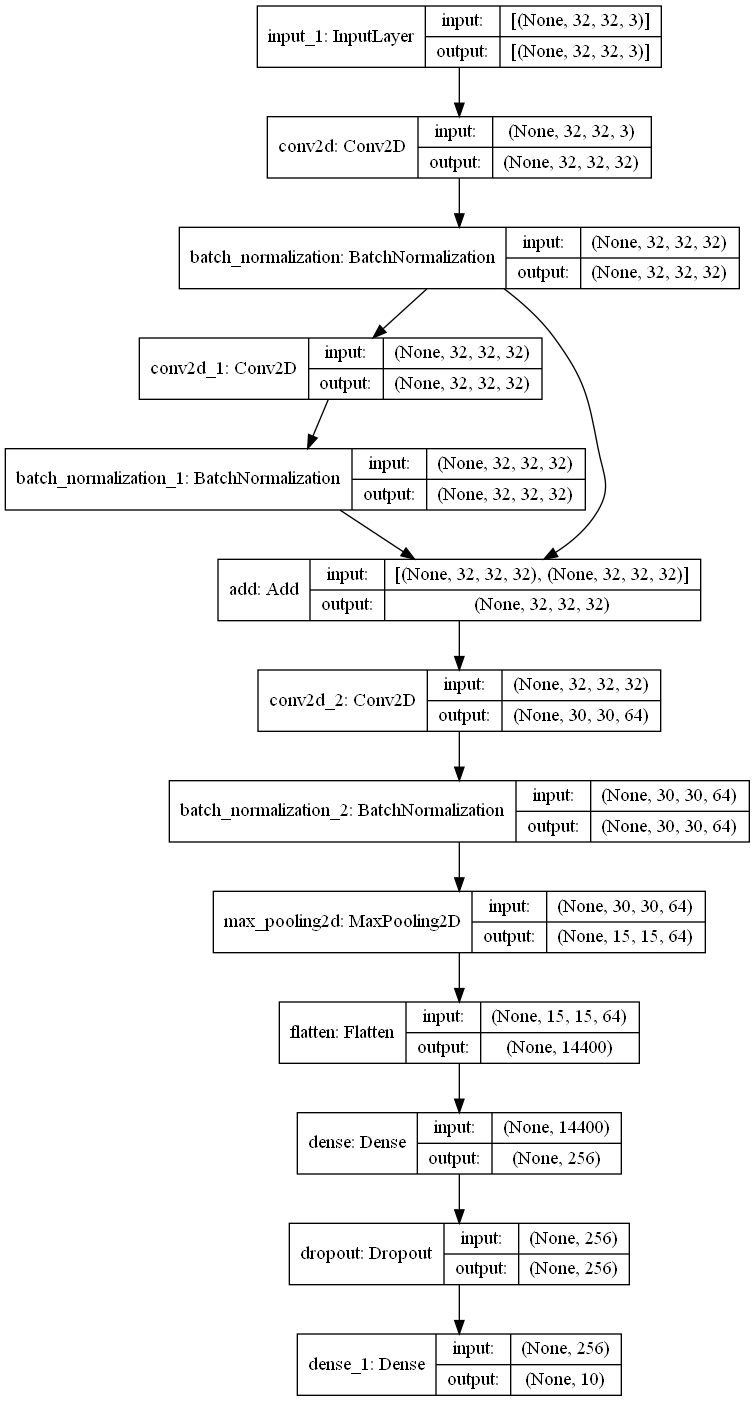
Later, we will use these two networks for training.

5, Network training

The part of network training includes:

• Define network
• Compile network
• Define callback function
• Define training process visualization function
• Training network
• Model saving

import utils                # Import the preprocessing library you just created
import net                  # Import the newly established network model library
from keras.callbacks import ReduceLROnPlateau, EarlyStopping
import matplotlib.pyplot as plt
import os
import datetime
# The following two lines represent calling CPU training. If you want to use GPU, you need to delete the following two lines
os.environ["CUDA_DEVICE_ORDER"] = "PCI_BUS_ID"
os.environ["CUDA_VISIBLE_DEVICES"] = "-1"

# Dataset loading
x_train, y_train, x_val, y_val, x_test, y_test = utils.load_data()

# Define network
conventional_model = net.conventional_model()
res_model = net.res_model()

# Compile network (define loss function, optimizer and evaluation index)
conventional_model.compile(loss='categorical_crossentropy', optimizer='adam', metrics=['accuracy'])
res_model.compile(loss='categorical_crossentropy', optimizer='adam', metrics=['accuracy'])

# Define the learning rate callback function (monitor the accuracy of the verification set and attenuate the learning rate according to the standard according to the set parameters)
learning_rate_reduction = ReduceLROnPlateau(monitor='val_acc', patience=2, verbose=1, factor=0.3, min_lr=0.00000001)
print('The current learning rate is:', learning_rate_reduction)
# Define the early stop callback function. When the accuracy of the monitored verification set is not optimized for 5 consecutive times, stop the network training and save the existing model
es = EarlyStopping(monitor='val_loss', patience=5)
# Callback function Union
callback = [learning_rate_reduction, es]

# Define the training process visualization function (training set loss, verification set loss, training set accuracy, verification set accuracy)
def show_train_history(train_history, train, validation):
    plt.plot(train_history.history[train])
    plt.plot(train_history.history[validation])
    plt.title('Train History')
    plt.ylabel(train)
    plt.xlabel('Epoch')
    plt.legend(['train', 'validation'], loc='best')
    plt.show()

def train_model(model):
    start_time = datetime.datetime.now()
    
    # Start network training (define training data and verification data, define training algebra, and define training batch size)
    train_history = model.fit(x_train, y_train, validation_data=(x_val, y_val),
                              epochs=30, batch_size=32, verbose=2, callbacks=[callback])

    elapsed_time = datetime.datetime.now() - start_time
    print('Training time:', elapsed_time)

    # Model saving
    model.save('res_model.h5')          # Modify the. h5 model name according to the network to be trained

    show_train_history(train_history, 'accuracy', 'val_accuracy')
    show_train_history(train_history, 'loss', 'val_loss')


if __name__ == '__main__':
    train_model(res_model)              # Select the network to train

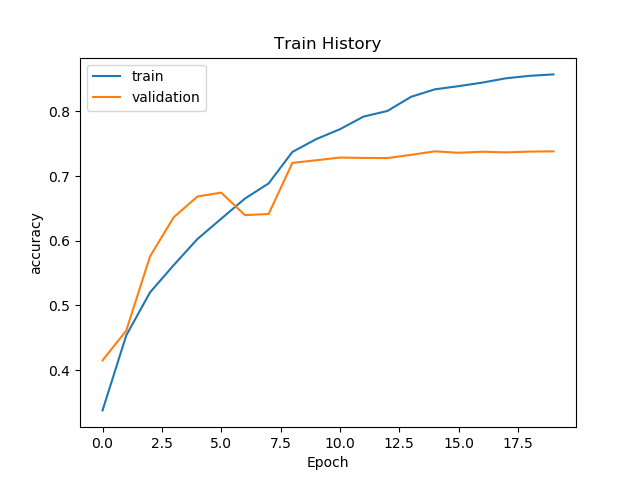
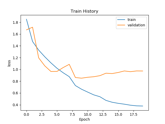
The training results of neural network with residual structure are as follows:

6, Network test

In step 5, we have trained the two networks and saved the corresponding models. Next, we can test the saved models.
In this part, there are the following steps:

• Load original dataset and preprocessed dataset
• Load the trained model
• Define prediction function
• Define the visualization function of prediction results
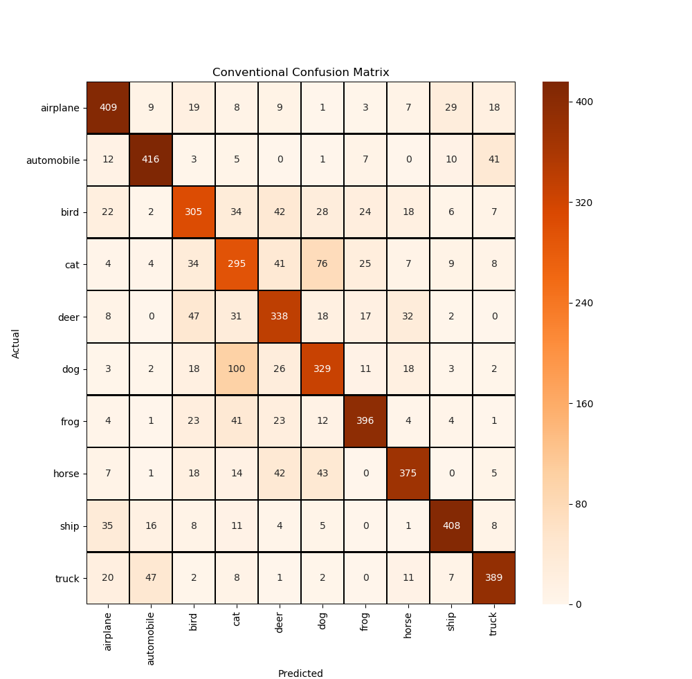
• Define confusion matrix

import utils
import matplotlib.pyplot as plt
import numpy as np
import keras
import pandas as pd
from sklearn.metrics import confusion_matrix
import seaborn as sns

# Load original dataset and preprocessed dataset
x_train_original, y_train_original, x_val_original, y_val_original, x_test_original, y_test_original = utils.val_set_alloc()
x_train, y_train, x_val, y_val, x_test, y_test = utils.load_data()

# Load the trained deep learning model
conventional_model = keras.models.load_model('conventional_model.h5')
res_model = keras.models.load_model('res_model.h5')

# Define prediction function
def model_predict(model):

    # For model prediction, the score includes the loss and accuracy of prediction results
    score = model.evaluate(x_test, y_test)
    print('Test loss:', score[0])           # Print test set loss
    print('Test accuracy:', score[1])       # Print test set precision

    # Test set result prediction (all test set prediction results are stored in predictions)
    predictions = model.predict(x_test)
    predictions = np.argmax(predictions, axis=1)            # The predicted single hot code is converted to conventional code, i.e. 0 1 2 3 4 5 6 7 8 9
    print('Prediction results of the first 20 pictures:', predictions[:20])

    return predictions


# Image visualization of prediction results
def mnist_visualize_multiple_predict(model, start, end, length, width):

    for i in range(start, end):
        plt.subplot(length, width, 1 + i)
        plt.imshow(x_test_original[i], cmap=plt.get_cmap('gray'))
        title_true = 'true=' + str(y_test_original[i])                  # Image reality label
        title_prediction = ',' + 'prediction' + str(predictions[i])     # Prediction results
        title = title_true + title_prediction
        plt.title(title)
        plt.xticks([])
        plt.yticks([])
    plt.show()

# Define confusion matrix
def confusion_matrix_visual(y_test_original, predictions):
    cm = confusion_matrix(y_test_original, predictions)
    cm = pd.DataFrame(cm)
    class_names = ['airplane', 'automobile', 'bird', 'cat', 'deer', 'dog', 'frog', 'horse', 'ship', 'truck']

    plt.figure(figsize=(10, 10))
    sns.heatmap(cm, cmap='Oranges', linecolor='black', linewidth=1, annot=True, fmt='', xticklabels=class_names,
                yticklabels=class_names)
    plt.xlabel("Predicted")
    plt.ylabel("Actual")
    plt.title("Conventional Confusion Matrix")
    plt.show()

if __name__ == '__main__':
    # Call the functions defined above
    predictions = model_predict(conventional_model)
    mnist_visualize_multiple_predict(conventional_model, start=0, end=9, length=3, width=3)
    confusion_matrix_visual(y_test_original, predictions)

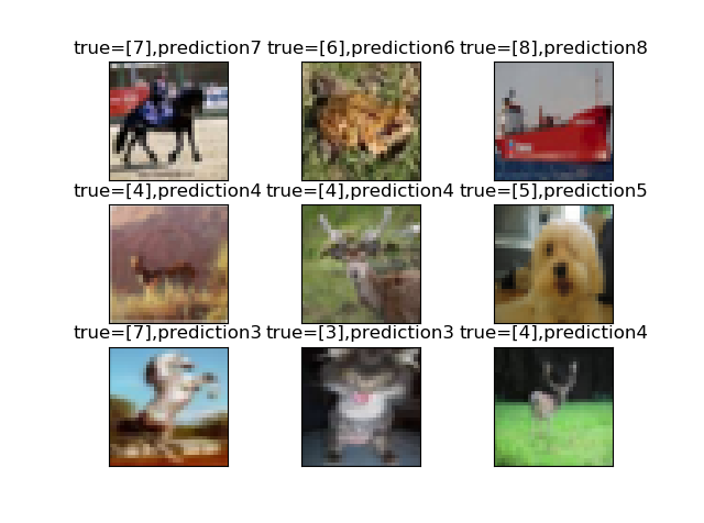
The prediction results of conventional CNN are as follows:

157/157 [==============================] - 3s 16ms/step - loss: 1.0221 - accuracy: 0.7410
Test loss: 1.0220750570297241
Test accuracy: 0.7409999966621399
 Prediction results of the first 20 pictures: [7 6 8 7 4 5 2 3 4 2 7 4 6 0 7 2 6 9 4 1]

The prediction results of CNN with residual structure are as follows:

157/157 [==============================] - 3s 16ms/step - loss: 1.0507 - accuracy: 0.7320
Test loss: 1.050661563873291
Test accuracy: 0.7319999933242798
 Prediction results of the first 20 pictures: [7 6 8 4 4 5 3 3 4 2 7 4 6 2 7 2 6 7 4 1]

7, Thinking and analysis

   we know that since he Kaiming proposed the residual network in 2015, it has greatly promoted the development of deep neural network. This is because the residual structure can prevent the gradient dispersion or gradient explosion caused by too deep network. So why is the accuracy of adding a jump connection in this experiment inferior to not adding it???
  this is because the residual network is suitable for deep networks. However, the network in this paper has only three layers of convolution, and the number of convolution cores is small, which can not reach the condition of deep. In addition, from the network training process diagram, the network is actually saturated in the eighth batch. At this time, the operation of reducing the learning rate and training step can not further optimize the neural network. In addition, the added jump connection will increase the amount of training, which will have a negative effect on the network!
   in conclusion, when setting up the network, we should not only consider the setting of super parameters, but also consider the bearing capacity of the network on the data set. Jump connections must be added in a reasonable place!!!

So how can we further optimize the network???

  we can use a multi-scale and multi branch network to extract the information of different receptive fields of the image by using a parallel structure in the shallow layer of the network. We can use 3 × 3,5 × In addition, attention mechanisms such as se can be added_ Block or CBAM, but note here that when adding attention, observe whether the focus area of the feature map is activated by the attention module. If it is not activated, it indicates that the addition of attention is invalid.

Finally, the SOTA of cifar10 hopes to be broken by you!!!