26 data analysis cases -- the second stop: Civil Aviation Customer Value Analysis Based on Hive

Environment required for experiment

• Python: Python 3.x；
• Hadoop2.7.2 environment;
• Hive2.2.0

Experimental background

People choose more and more travel modes, such as aircraft, high-speed rail, cars, ships, etc. in particular, aircraft is known as the most safe and efficient means of transportation so far. The problem of how airlines can provide high-quality services to customers and maximize their interests always puzzles airlines. In order to solve one of the problems, they can group customers by using Hive, For example, important retention customers, important development customers, important retention customers, general customers and low value customers, and then specify corresponding preferential policies according to different customer groups to maximize benefits.

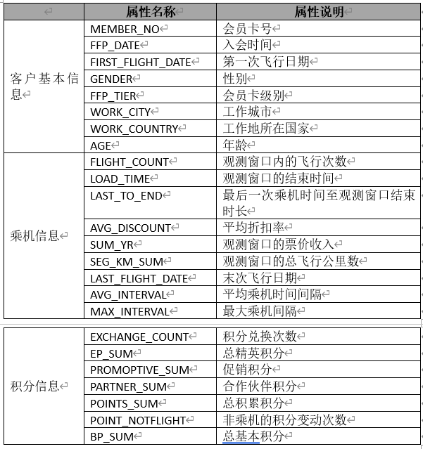
Data description

Necessary knowledge

1. SELECT... FROM statement

The SELECT... FROM statement is the basic statement in the query. It can query the data in the specified table and filter the columns in the table. In addition, in order to easily distinguish different tables in multi table Association queries, the SELECT... FROM statement can also execute aliases for tables in the query statement (the current query will expire after the end of the current query and the original table attributes of the table will not be). The SELECT... FROM syntax is as follows.

SELECT select_list FROM table_source 

The parameter name is as follows:

• select_list: select_ List represents the list of column names contained in the query results. Columns are separated by commas. If you need to list all fields in the table, you can use "*" instead.
• table_source: the table to query.

2. WHERE condition query

SELECT... FROM statement can list all records in the table. If you want to query the matching records according to some specific conditions, you need to use the WHERE clause. The WHERE statement is usually used together with this expression. In case of multiple conditions, multiple expressions can be connected through AND OR. When the result of the expression returns True, the corresponding column value is output.

SELECT select_list FROM table_source WHERE search_condition

3. JOIN join query

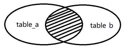
(1) INNER JOIN

Inner join query refers to retaining the data that exists in both connected tables and meets the join criteria. The inner join syntax is as follows.

SELECT select_list FROM table_source a JOIN table_source b ON a.col=b.col

The internal connection principle is shown in the figure.

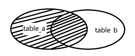
(2)LEFT JOIN

The left outer connection refers to the association based on the left table, and returns all records in the left table and those in the right table that meet the connection conditions. The records that do not match are replaced by null in the result. The syntax is as follows.

SELECT select_list FROM table_source a LEFT JOIN table_source b ON a.col=b.col

The left connection principle is shown in the figure.

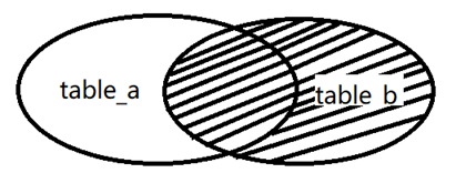
(3)RIGHT JOIN

The effect of the right outer join method is opposite to that of the left outer join method. The right outer join refers to the right table, and returns all records in the right table and records in the left table that meet the join conditions. The left and right tables are defined relative to the join clause. When using the left outer join, you only need to change the position of the two tables to realize the right outer join function. Similarly, the right outer connection can also achieve the effect of the left outer connection. The syntax of right outer connection is as follows.

SELECT select_list FROM table_source a LEFT JOIN table_source b ON a.col=b.col

The principle of right external connection is shown in the figure.

(4)FULL JOIN

External connection refers to connecting all the data in two tables. If there is no corresponding number, it will be empty. The external connection syntax is as follows.

SELECT select_list FROM table_source a FULL OUTER JOIN table_source b ON a.col=b.col

The principle of all external links is shown in the figure.

4. Aggregate function

The aggregation function is special. It can calculate multiple rows of data, such as summation, average value, etc. Aggregate functions are often used with GROUP BY grouping statements. The aggregate functions commonly used in Hive are shown in the following table.

function	describe
count(*)	Counting function
sum(col)	Summation function
avg(col)	Mean value function
min(col)	Minimum function
max(col)	Maximum function

5. Set function

The values stored in columns in Hive data warehouse can be array or map data. For these two special types, Hive provides set functions to process such data. Set functions can return set length, array length, key value or value value in key value pair type, etc. set functions are shown in the following table.

function	explain
size(Map<K.V>)	Returns the length of the map type
map_keys(Map<K.V>)	Returns all key s in the map
map_values(Map<K.V>)	Returns all value s in the map
array_contains(Array, value)	If the Array contains value, return true. Otherwise, false is returned
sort_array(Array)	Sorts the array in natural order and returns

6. Date function

As the name suggests, a date function refers to a function that specifically operates on data representing time. The commonly used date format in daily life and production is "yyyy MM DD HH: mm: SS". This is because the format takes up too many characters or is too complex to meet all application scenarios. When it is necessary to convert date data, a date function can be used, Common date functions are shown in table.

function	explain
from_unixtime	Converts the timestamp to the specified format
unix_timestamp	According to different parameters, you can remove the local timestamp or convert the date to timestamp
to_date	Return to mm / DD / yy
year	Return year section
month	Return to month section
day	Return day section
hour	Return to the hours section
minute	Return to the minutes section
second	Return to the second part
datediff	Returns the number of days from the start time to the end time
date_add	Add the specified number of days to the specified date
date_sub	Subtract the specified number of days from the specified date
current_date	Returns the current time and date
date_format	Returns the time in the specified format

7. String function

The main function of string function is to process string type data, such as case conversion, string format conversion, space removal and string interception. Common string functions are shown in the table.
Function description
format_number converts the value X to a "#, ####, ###, ##. ##" format string
get_json_object extract JSON object
lower capital to lowercase
upper lowercase to uppercase
ltrim removes spaces before strings
rtrim removes spaces after strings
Split split split string
substr intercept string

Data package

Link: https://pan.baidu.com/s/1Uzx5g2r54k9Q2PYK5_DlTQ 
Extraction code: irq2

Experimental steps

Step 1: load the dataset

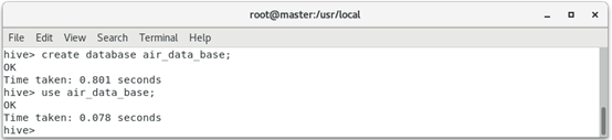
1. Create a named air in Hive_ data_ Base database.

hive > create database air_data_base;
hive > use air_data_base;

The operation result is:

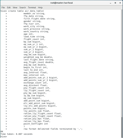
2. The data created above is painstakingly named air_data_table.

hive> create table air_data_table(
            member_no string,
            ffp_date string,
            first_flight_date string,
            gender string,
            ffp_tier int,
            work_city string,
            work_province string,
            work_country string,
            age int,
            load_time string,
            flight_count int,
            bp_sum bigint,
            ep_sum_yr_1 int,
            ep_sum_yr_2 bigint,
            sum_yr_1 bigint,
            sum_yr_2 bigint,
            seg_km_sum bigint,
            weighted_seg_km double,
            last_flight_date string,
            avg_flight_count double,
            avg_bp_sum double,
            begin_to_first int,
            last_to_end int,
            avg_interval float,
            max_interval int,
            add_points_sum_yr_1 bigint,
            add_points_sum_yr_2 bigint,
            exchange_count int,
            avg_discount float,
            p1y_flight_count int,
            l1y_flight_count int,
            p1y_bp_sum bigint,
            1y_bp_sum bigint,
            ep_sum bigint,
            add_point_sum bigint,
            eli_add_point_sum bigint,
            l1y_eli_add_points bigint,
            points_sum bigint,
            l1y_points_sum float,
            ration_l1y_flight_count float,
            ration_p1y_flight_count float,
            ration_p1y_bps float,
            ration_l1y_bps float,
            point_notflight int
            )
            row format delimited fields terminated by ',';

The operation result is:

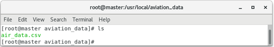
3. Create a file named aviation in the / usr/local directory_ Data and will be named air_ data. The CSV data set is uploaded to this directory, and the result is:

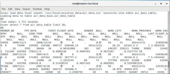
4. Load the data into a file named air_ data_ In the data table of table

hive > load data local inpath '/usr/local/aviation_data/air_data.csv' overwrite into table air_data_table;
hive> select * from air_data_table limit 10;

The operation result is:

Step 2: data analysis

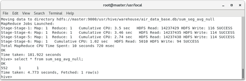
1. Make statistics on the null value records of the fare revenue (SUM_YR_1), total flight kilometers (SEG_KM_SUM) and average discount rate (AVG_DISCOUNT) of the observation window, and save the results to the table named sum_seg_avg_null.

hive > create table sum_seg_avg_null as select * from
(select count(*) as sum_yr_1_null_count from air_data_table where sum_yr_1 is null)
sum_yr_1,
(select count(*) as seg_km_sum_null from air_data_table where seg_km_sum is null)
seg_km_sum,
(select count(*) as avg_discount_null from air_data_table where avg_discount is null)
avg_discount;
hive> select * from sum_seg_avg_null;

The operation result is:

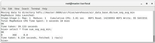
2. Use the select statement to count air_ data_ Sum of observation window in table_ YR_ The minimum value sum_seg_avg_min in column 1 (fare revenue), SEG_KM_SUM (total flight kilometers) and AVG_DISCOUNT (average discount rate) is shown in the table.

hive (default)> create table sum_seg_avg_min as select
            min(sum_yr_1) sum_yr_1,
            min(seg_km_sum) seg_km_sum,
            min(avg_discount) avg_discount
            from air_data_table;
hive (default)> select * from sum_seg_avg_min;

The operation result is:

Step 3: data cleaning

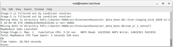
1. Through the data analysis of the above two steps, it is not difficult to see that the data contains some missing data, but the missing part only occupies a small part of the overall data and will not affect the final data analysis results. Therefore, the missing value is directly filtered out here. The filtered data includes records with empty ticket price, records with an average discount rate of 0.0, ticket price of 0 Records where the average discount rate is not 0 and the total flight kilometers are greater than 0.

hive (default)> create table sum_yr_1_notnull as
select * from air_data_table where
            sum_yr_1 is not null;
hive (default)> create table avg_discount_not_0 as select *
            from sum_yr_1_notnull where 
            avg_discount <> 0;
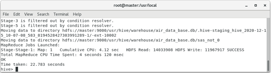
hive (default)> create table sas_not_0 as
             select * from avg_discount_not_0
             where !(sum_yr_1=0 and avg_discount <> 0
             and seg_km_sum > 0);

The operation result is:
Filter out the records with empty ticket price

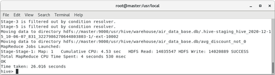
Filter records with an average discount rate of 0.0

Filter the records where the fare is 0, the average discount rate is not 0, and the total flight kilometers are greater than 0

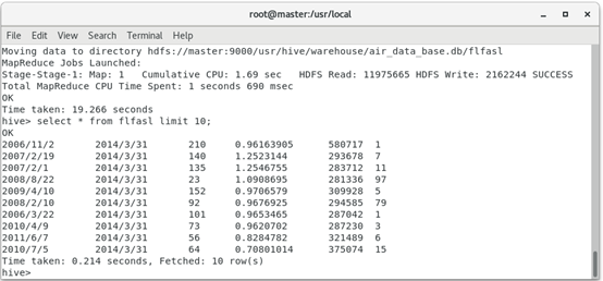
2. In order to facilitate the establishment of LRFMC model, six related attributes need to be selected from the cleaned data, namely LOAD_TIME,FFP_DATE,LAST_TO_END,FLIGHT_COUNT,SEG_KM_SUM,AVG_DISCOUNT.

hive> create table flfasl as select ffp_date,load_time,flight_count,avg_discount,seg_km_sum,last_to_end from sas_not_0;
hive> select * from flfasl limit 10;

The operation result is:

3. Carry out data conversion and convert the data into an appropriate format to meet the needs of mining tasks and algorithms. In this task, the data conversion algorithms are as follows (the algorithms in this part are only for value analysis in the aviation field).
The five indexes and algorithms for constructing LRFMC are as follows.
(1) L structure: the number of months from the membership time to the end of the observation window = the end time of the observation window - Membership time [unit: month]. The formula in this task is as follows.

L = LOAD_TIME - FFP_DATE

(2) Structure of R: the number of months from the end of the observation window when the customer last took the company's aircraft = the length of time from the last flight time to the end of the observation window [unit: month]. The formula in this task is as follows.

R = LAST_TO_END

(3) F structure: the number of times the customer takes the company's aircraft in the re observation window = the number of flights in the observation window [unit: Times]. The formula in this task is as follows.

F = FLIGHT_COUNT

(4) M structure: the accumulated flight mileage of the company during the customer's re observation time = the total flight kilometers of the observation window [unit: km]. The formula in this task is as follows.

M = SEG_KM_SUM

(5) C structure: the average value of the discount coefficient corresponding to the class taken by the customer during the observation time = the average discount rate [unit: none]. The formula in this task is as follows.

C = AVG_DISCOUNT

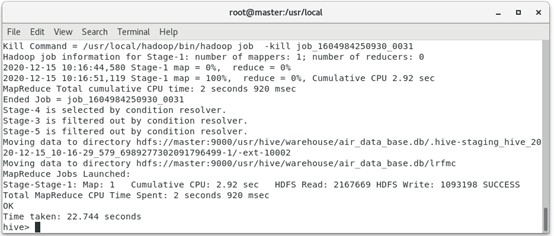
Calculate the data after data protocol according to the above formula to obtain LRFMC.

hive> create table lrfmc as select
round((unix_timestamp(LOAD_TIME,'yyyy/MM/dd')-unix_timestamp(FFP_DATE,'>yyyy/MM/dd'))/(30*24*60*60),2) as l,
round(last_to_end/30,2) as r,
FLIGHT_COUNT as f,
SEG_KM_SUM as m,
round(AVG_DISCOUNT,2) as c
from flfasl;

The operation result is:

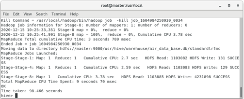
4. Standardize the data. The formula is standardized value = (x - min(x))/(max(x) - min(x)). Save the standardized data to the table named "standardlrfmc".

hive> create table standardlrfmc as
     select (lrfmc.l-minlrfmc.l)/(maxlrfmc.l-minlrfmc.l) as l,
      (lrfmc.r-minlrfmc.r)/(maxlrfmc.r-minlrfmc.r) as r,
     (lrfmc.f-minlrfmc.f)/(maxlrfmc.f-minlrfmc.f) as f,
     (lrfmc.m-minlrfmc.m)/(maxlrfmc.m-minlrfmc.m) as m,
     (lrfmc.c-minlrfmc.c)/(maxlrfmc.c-minlrfmc.c) as c
     from lrfmc,
     (select max(l) as l,max(r) as r,max(f) as f,max(m) as m,max(c) as c from lrfmc) as maxlrfmc,
(select min(l) as l,min(r) as r,min(f) as f,min(m) as m,min(c) as c from lrfmc) as minlrfmc;

The operation result is:

5. Export the standardized data to the local standard lrfmc CSV and use commas as as separators.

[root@master ~]# hive -e "insert overwrite local directory '/usr/local/standardlrfmc' row format delimited fields terminated by ',' select * from air_data.standardlrfmc;"
[root@master ~]# cd /usr/local/standardlrfmc
[root@master standardlrfmc]# ls
[root@master standardlrfmc]# mv 000000_0 standardlrfmc.csv
[root@master standardlrfmc]# ls

Step 4: customer classification

1. According to the business logic, customers are roughly divided into five categories. With k=5 and the standardized data, the clustering centers of these five customer groups can be calculated by using the previously established Kmeans model.

>>> import pandas as pd
>>> import numpy as np
>>> from sklearn.cluster import KMeans
>>> dt=pd.read_csv("/usr/local/standardlrfmc/standardlrfmc.csv",encoding='UTF-8')
>>> dt.columns=['L','R','F','M','C']
>>> model=KMeans(n_clusters=5)
>>> model.fit(dt)
>>> r1=pd.Series(model.labels_).value_counts()
>>> r2=pd.DataFrame(model.cluster_centers_)
>>> r=pd.concat([r2,r1],axis=1)
>>> r.columns=list(dt.columns)+['Clustercategory']
>>> r

The operation result is:

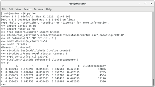
According to the clustering center results and the business logic of airlines, the following results can be obtained:
 customer group 1 has the largest C attribute, which can be defined as important retention customers;
 Customers 2 has the largest L attribute and can be defined as important development customers.
 customer group 3 is the smallest in F and M attributes and can be defined as low-value customers;
 customer group 4 has the largest L attribute and can be defined as general customers;
 Customers 5 has the smallest F and M attributes and can be defined as low-value customers;

Follow up cases are continuously updated

01 crown size query system
02 civil aviation customer value analysis
03 pharmacy sales data analysis
04 browser traffic access offline log collection and processing
05 Muke network data acquisition and processing
06 Linux operating system real-time log collection and processing
07 medical industry case - Analysis of dialectical association rules of TCM diseases
08 education industry case - Analysis of College Students' life data
10 entertainment industry case - advertising revenue regression prediction model
11 network industry case - website access behavior analysis
12 retail industry case - real time statistics of popular goods in stores
13 visualization of turnover data
14 financial industry case - financial data analysis based on stock information of listed companies and its derivative variables
15 visualization of bank credit card risk data
Operation analysis of 16 didi cities
17 happiness index visualization
18 employee active resignation warning model
19 singer recommendation model
202020 novel coronavirus pneumonia data analysis
Data analysis of 21 Taobao shopping Carnival
22 shared single vehicle data analysis
23 face detection system
24 garment sorting system
25 mask wearing identification system
26 imdb movie data analysis