Convolutional neural network (CNN)
Learning objectives
- Understand the composition of convolutional neural network
- Know the principle and calculation process of convolution
- Understand the function and calculation process of pooling
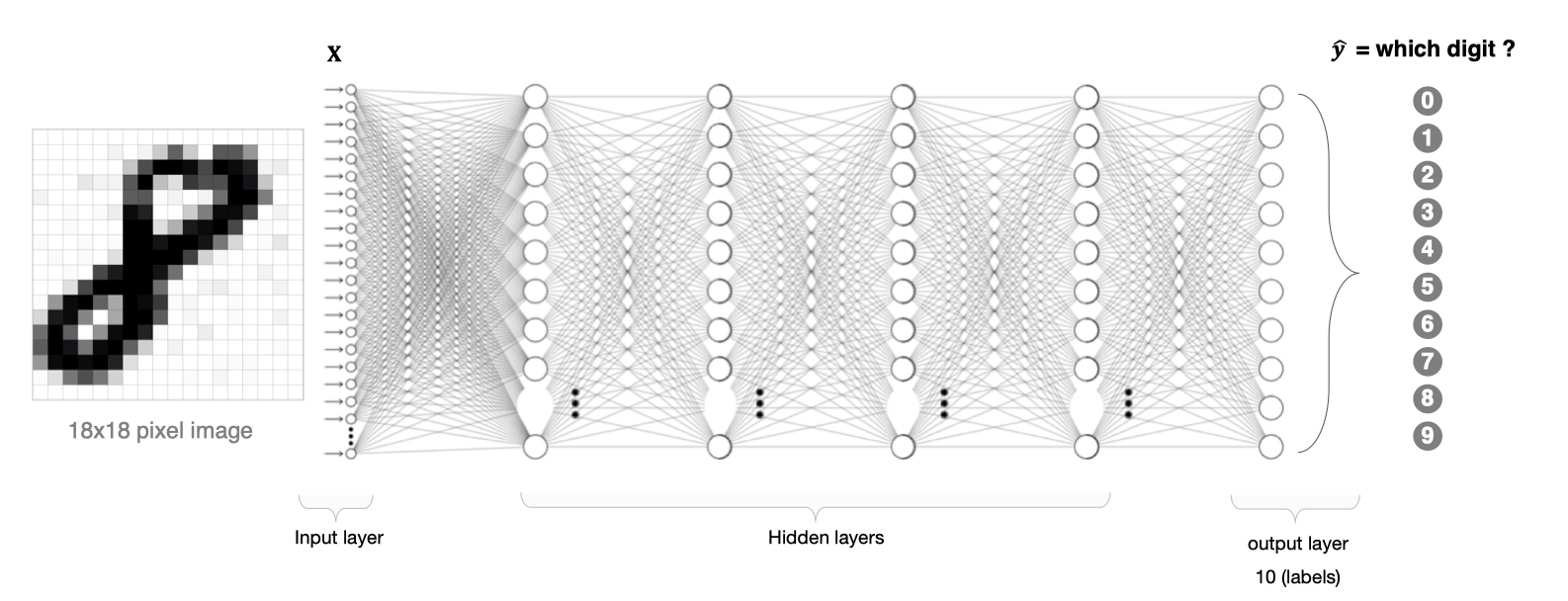
There are two problems in image processing using fully connected neural network:
- The amount of data to be processed is large and the efficiency is low
If we deal with a 1000 × 1000 pixel picture with the following parameters:
1000×1000×3=3,000,000
Processing such a large amount of data is very resource consuming
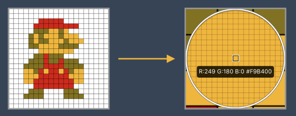
- In the process of image dimension adjustment, it is difficult to retain the original features, resulting in the low accuracy of image processing
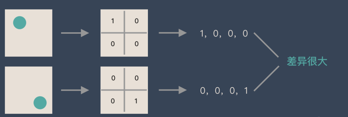
If a circle is 1 and no circle is 0, different positions of the circle will produce completely different data expressions. However, from the perspective of the image, the content (essence) of the image has not changed, but the position has changed. Therefore, when we move the object in the image, the results obtained by lifting with full connection will be very different, which does not meet the requirements of image processing.
Composition of CNN network
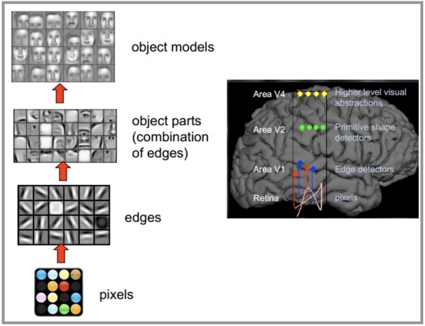
CNN network is inspired by the human visual nervous system. The principle of human vision: start with the intake of the original signal (the pupil ingests Pixels), then do preliminary processing (some cells in the cerebral cortex find the edge and direction), and then abstract (the brain determines that the shape of the object in front of you is round), Then further abstraction (the brain further determines that the object is a face). The following is an example of human brain face recognition:
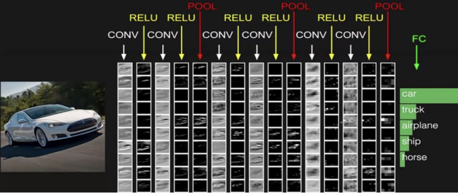
CNN network is mainly composed of three parts: convolution layer, pooling layer and full connection layer, in which convolution layer is responsible for extracting local features in the image; The pool layer is used to greatly reduce the parameter order (dimension reduction); The full connection layer is similar to the part of artificial neural network, which is used to output the desired results.

The whole CNN network structure is shown in the figure below:
Convolution layer
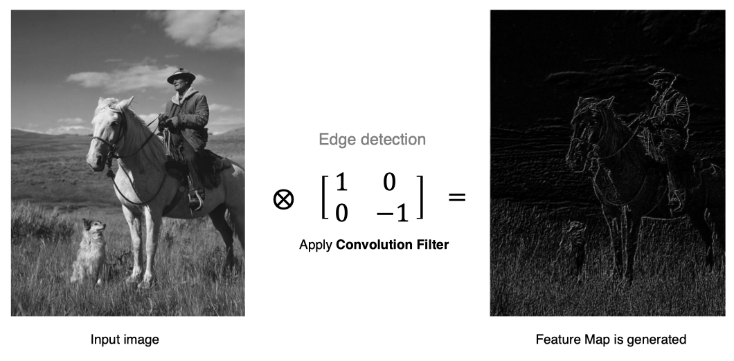
The convolution layer is the core module in the convolution neural network. The purpose of the convolution layer is to extract the features of the input feature map. As shown in the figure below, the convolution core can extract the edge information in the image.
Calculation method of convolution
How is convolution calculated?
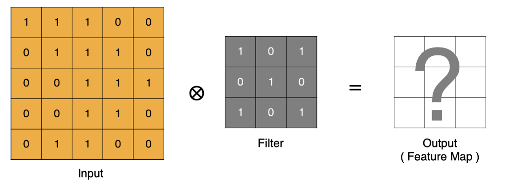
Convolution is essentially a dot product between the filter and the local area of the input data.
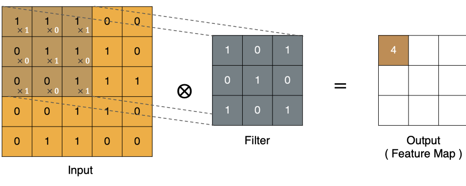
Calculation method of points in the upper left corner:

Similarly, other points can be calculated to obtain the final convolution result,
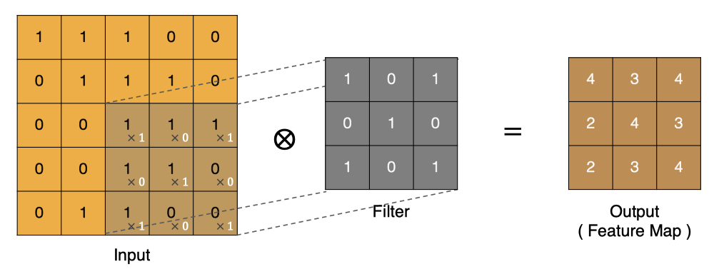
The last point is calculated as follows:

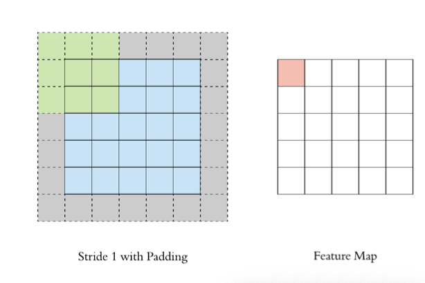
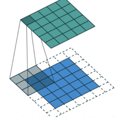
padding
In the above convolution process, the feature image is much smaller than the original image. We can pad around the original image to ensure that the size of the feature image remains unchanged in the convolution process.
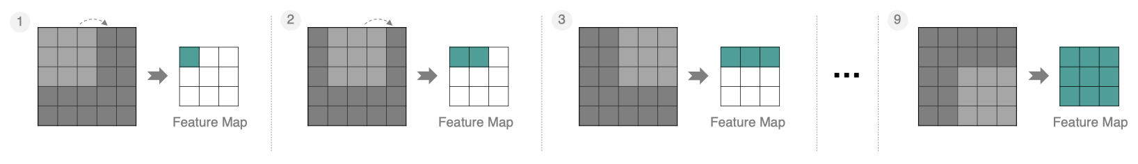
Stripe (step size)
Move the convolution kernel according to the step size of 1, and the calculated characteristic diagram is as follows:
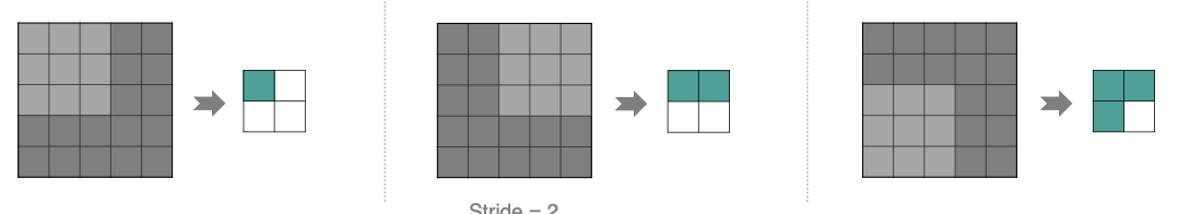
If we increase the stripe, for example, set it to 2, we can also extract the feature map, as shown in the following figure:
Multichannel convolution
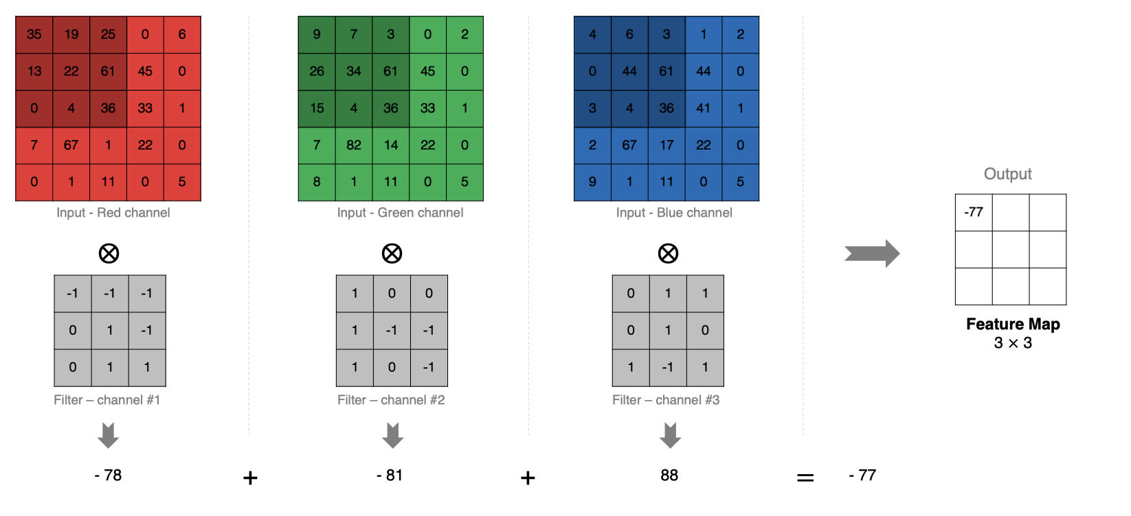
In practice, images are composed of multiple channels. How do we calculate convolution?
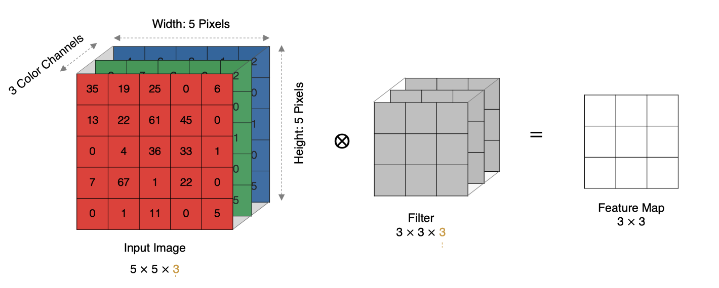
The calculation method is as follows: when the input has multiple channels (for example, the picture can have three RGB channels), the convolution core needs to have the same number of channels. Each convolution core channel is convoluted with the corresponding channel of the input layer, and the convolution results of each channel are added according to the phase to obtain the final Feature Map
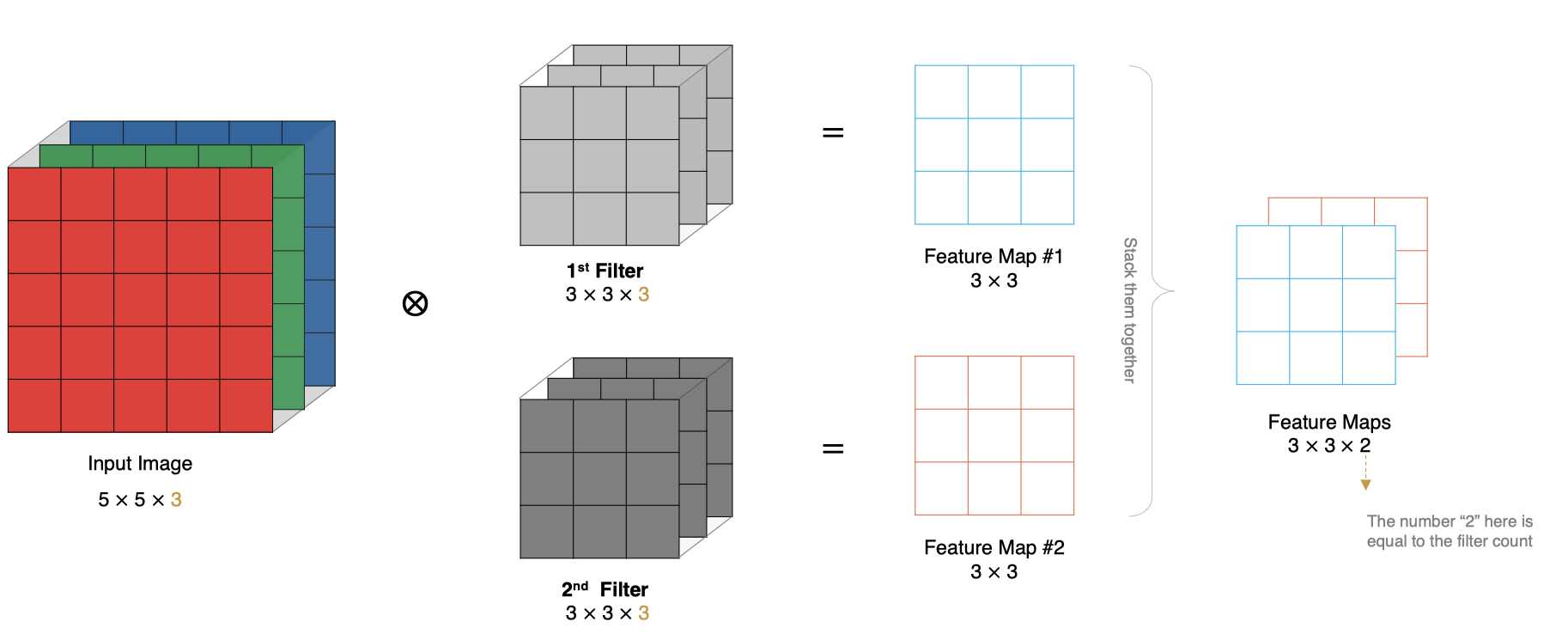
Multi convolution kernel convolution
How to calculate if there are multiple convolution kernels? When there are multiple convolution cores, each convolution core learns different features and generates a Feature Map containing multiple channels. For example, the following figure has two filter s, so the output has two channels.
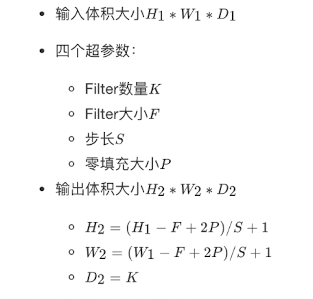
Size feature map
The size of the output characteristic graph is closely related to the following parameters: * Size: convolution kernel / filter size, which is generally selected as an odd number, such as 1 * 1, 3 * 3, 5 * 5 * padding: zero filling method * stripe: step size
The calculation method is shown in the figure below:
If the input characteristic diagram is 5x5, the convolution kernel is 3x3, and the additional padding is 1, the output size is:
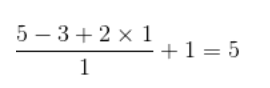
As shown in the figure below:
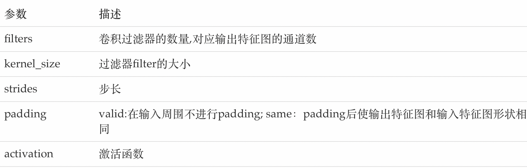
In TF Implementation and application of convolution kernel in keras
tf.keras.layers.Conv2D(
    filters, kernel_size, strides=(1, 1), padding='valid',
     activation=None
)
The main parameters are described as follows:
Pooling layer
The pooling layer reduces the input dimension of the subsequent network layer, reduces the size of the model, improves the calculation speed, improves the robustness of the Feature Map and prevents over fitting,
It mainly subsamples the feature map learned by the convolution layer, which is mainly composed of two methods
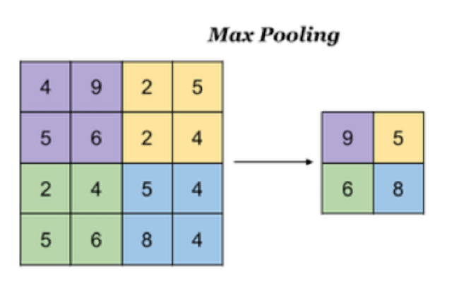
Maximum pooling
- Max Pooling, which takes the maximum value in the window as the output. This method is widely used.
In TF The methods implemented in keras are:
tf.keras.layers.MaxPool2D(
    pool_size=(2, 2), strides=None, padding='valid'
)
Parameters:
pool_size: Size of pooled window

strides: The step size of window movement, which is 1 by default

padding: Whether to fill or not. The default is not to fill
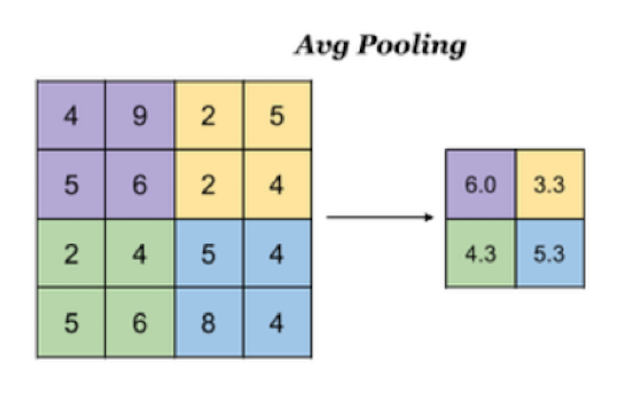
Average pooling
Avg Pooling, take the average value of all values in the window as the output
In TF The methods to implement pooling in keras are:
tf.keras.layers.AveragePooling2D(
    pool_size=(2, 2), strides=None, padding='valid'
)
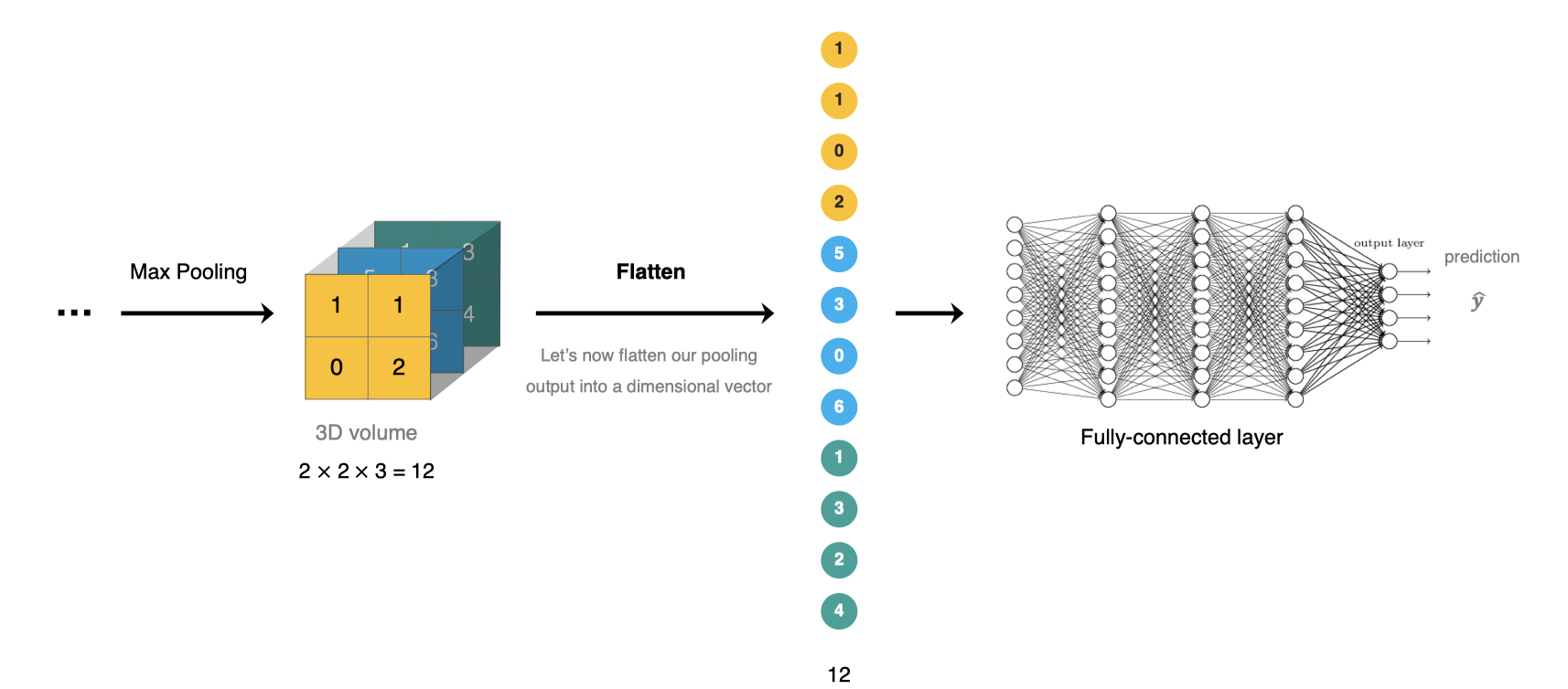
Full connection layer
The full connection layer is located at the end of CNN network. After feature extraction of convolution layer and dimension reduction of pooling layer, the feature map is transformed into one-dimensional vector and sent to the full connection layer for classification or regression.
In TF TF is used in the full connection layer of keras keras. Dense implementation.
Construction of convolutional neural network
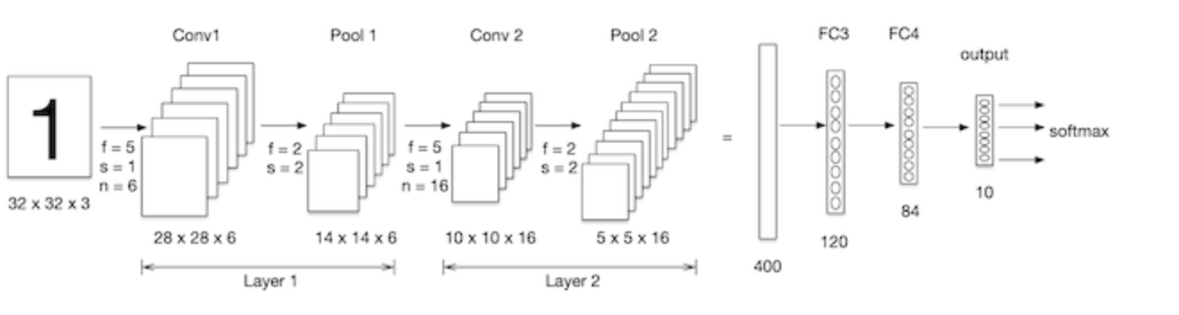
We build a convolutional neural network and process it on the mnist data set, as shown in the figure below: LeNet-5 is a relatively simple convolutional neural network. The input two-dimensional image first passes through the convolution layer, the pooling layer, and then through the full connection layer. Finally, softmax classification is used as the output layer.
Import Kit:
import tensorflow as tf
# data set
from tensorflow.keras.datasets import mnist
Data loading
Consistent with the case of neural network, first load the data set:
(train_images, train_labels), (test_images, test_labels) = mnist.load_data()
data processing
The input requirements of convolutional neural network are: N H W C, which are the number of pictures, the height of pictures, the width of pictures and the channel of pictures respectively. Because it is a gray image, the channel is 1
# Data processing: num,h,w,c
# Training set data
train_images = tf.reshape(train_images, (train_images.shape[0],train_images.shape[1],train_images.shape[2], 1))
print(train_images.shape)
# Test set data
test_images = tf.reshape(test_images, (test_images.shape[0],test_images.shape[1],test_images.shape[2], 1))
The result is:
(60000, 28, 28, 1)
Model building
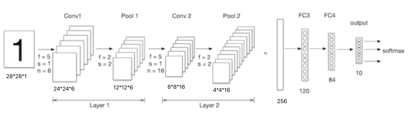
The two-dimensional image input by the Lenet-5 model first passes through the convolution layer, the pool layer, and then through the full connection layer. Finally, the softmax classification is used as the output layer. The model is constructed as follows:
# model building
net = tf.keras.models.Sequential([
    # Convolution layer: Six 5 * 5 convolution kernels with sigmoid activation
      tf.keras.layers.Conv2D(filters=6,kernel_size=5,activation='sigmoid',input_shape=  (28,28,1)),
    # Maximum pooling
    tf.keras.layers.MaxPool2D(pool_size=2, strides=2),
    # Convolution layer: 16 convolution cores of 5 * 5 with sigmoid activation
    tf.keras.layers.Conv2D(filters=16,kernel_size=5,activation='sigmoid'),
    # Maximum pooling
    tf.keras.layers.MaxPool2D(pool_size=2, strides=2),
    # Adjust dimension to 1D data
    tf.keras.layers.Flatten(),
    # Full convolution, activate sigmoid
    tf.keras.layers.Dense(120,activation='sigmoid'),
    # Full convolution, activate sigmoid
    tf.keras.layers.Dense(84,activation='sigmoid'),
    # Full convolution, activate softmax
    tf.keras.layers.Dense(10,activation='softmax')

])
We passed net Summary() to view the network structure:
Model: "sequential_11"
_________________________________________________________________
Layer (type)                 Output Shape              Param #
=================================================================
conv2d_4 (Conv2D)            (None, 24, 24, 6)         156
_________________________________________________________________
max_pooling2d_4 (MaxPooling2 (None, 12, 12, 6)         0
_________________________________________________________________
conv2d_5 (Conv2D)            (None, 8, 8, 16)          2416
_________________________________________________________________
max_pooling2d_5 (MaxPooling2 (None, 4, 4, 16)          0
_________________________________________________________________
flatten_2 (Flatten)          (None, 256)               0
_________________________________________________________________
dense_25 (Dense)             (None, 120)               30840
_________________________________________________________________
dense_26 (Dense)             (None, 84)                10164

dense_27 (Dense)             (None, 10)                850
=================================================================
Total params: 44,426
Trainable params: 44,426
Non-trainable params: 0
______________________________________________________________
Parameter calculation
The size of the handwritten digital input image is 28x28x1. As shown in the figure below, let's look at the parameter quantity of the next convolution layer:
The convolution kernel in conv1 is 5x5x1, the number of convolution kernels is 6, and each convolution kernel has a bias, so the parameter quantity is: 5x5x1x6+6=156.
The convolution kernel in conv2 is 5x5x6, the number of convolution kernels is 16, and each convolution kernel has a bias, so the parameter quantity is 5x5x6x16+16 = 2416.
Model compilation
Set optimizer and loss function:
# optimizer
optimizer = tf.keras.optimizers.SGD(learning_rate=0.9)
# Model compilation: loss function, optimizer and evaluation index
net.compile(optimizer=optimizer,
              loss='sparse_categorical_crossentropy',
              metrics=['accuracy'])
model training
Model training:
# model training
net.fit(train_images, train_labels, epochs=5, validation_split=0.1)
Training process:
Epoch 1/5
1688/1688 [==============================] - 10s 6ms/step - loss: 0.8255 - accuracy: 0.6990 - val_loss: 0.1458 - val_accuracy: 0.9543
Epoch 2/5
1688/1688 [==============================] - 10s 6ms/step - loss: 0.1268 - accuracy: 0.9606 - val_loss: 0.0878 - val_accuracy: 0.9717
Epoch 3/5
1688/1688 [==============================] - 10s 6ms/step - loss: 0.1054 - accuracy: 0.9664 - val_loss: 0.1025 - val_accuracy: 0.9688
Epoch 4/5
1688/1688 [==============================] - 11s 6ms/step - loss: 0.0810 - accuracy: 0.9742 - val_loss: 0.0656 - val_accuracy: 0.9807
Epoch 5/5
1688/1688 [==============================] - 11s 6ms/step - loss: 0.0732 - accuracy: 0.9765 - val_loss: 0.0702 - val_accuracy: 0.9807
Model evaluation
# Model evaluation
score = net.evaluate(test_images, test_labels, verbose=1)
print('Test accuracy:', score[1])
Output is:
313/313 [==============================] - 1s 2ms/step - loss: 0.0689 - accuracy: 0.9780
Test accuracy:  0.9779999852180481
Compared with the use of fully connected network, the accuracy is much improved.
summary
- Composition of convolutional neural network
Convolution layer, pooling layer, full connection layer
- Convolution layer
Convolution calculation process, stripe, padding
- Pool layer
Maximum pooling and average pooling
- Implementation and construction program of CNN structure