DataWhale teamed up to learn GNN task6
Reference:[ DataWhale GNN learning materials],What are weisfeiler Lehman (WL) algorithm and WL Test- Zhihu (zhihu.com),Weisfeiler Leman test and WL subtree kernel_kingloon blog - CSDN blog
Graph eigen learning of graph isomorphic networks
Implementation of graph representation network based on graph isomorphic network (GIN)
Graph feature learning based on graph isomorphic network mainly includes the following two processes:
- Firstly, the node representation is calculated
- Secondly, Graph Pooling or Graph Readout is done for the representation of each node on the graph to obtain Graph Representation
Graph representation module based on graph isomorphic network
GINNodeEmbedding module embeds each node in the graph to get the representation of the node, then pools the representation of the node to get the representation of the graph, and finally uses a layer of linear transformation to get the representation of the graph. The code implementation is as follows:
import torch
from torch import nn
from torch_geometric.nn import global_add_pool, global_mean_pool, global_max_pool, GlobalAttention, Set2Set
from gin_node import GINNodeEmbedding

class GINGraphRepr(nn.Module):

    def __init__(self, num_tasks=1, num_layers=5, emb_dim=300, residual=False, drop_ratio=0, JK="last", graph_pooling="sum"):
        """GIN Graph Pooling Module
        Args:
            num_tasks (int, optional): number of labels to be predicted. Defaults to 1 (Controls the dimension of graph representation).
            num_layers (int, optional): number of GINConv layers. Defaults to 5.
            emb_dim (int, optional): dimension of node embedding. Defaults to 300.
            residual (bool, optional): adding residual connection or not. Defaults to False.
            drop_ratio (float, optional): dropout rate. Defaults to 0.
            JK (str, optional): The optional values are"last"and"sum". choose"last",Only take the embedding of the last layer of nodes, and select"sum"Embedding and summation of nodes in each layer.
            graph_pooling (str, optional): pooling method of node embedding. The optional values are"sum","mean","max","attention"and"set2set".  Defaults to "sum".

        Out:
            graph representation
        """
        super(GINGraphPooling, self).__init__()

        self.num_layers = num_layers
        self.drop_ratio = drop_ratio
        self.JK = JK
        self.emb_dim = emb_dim
        self.num_tasks = num_tasks

        if self.num_layers < 2:
            raise ValueError("Number of GNN layers must be greater than 1.")

        self.gnn_node = GINNodeEmbedding(num_layers, emb_dim, JK=JK, drop_ratio=drop_ratio, residual=residual)

        # Pooling function to generate whole-graph embeddings
        if graph_pooling == "sum":
            self.pool = global_add_pool
        elif graph_pooling == "mean":
            self.pool = global_mean_pool
        elif graph_pooling == "max":
            self.pool = global_max_pool
        elif graph_pooling == "attention":
            self.pool = GlobalAttention(gate_nn=nn.Sequential(
                nn.Linear(emb_dim, emb_dim), nn.BatchNorm1d(emb_dim), nn.ReLU(), nn.Linear(emb_dim, 1)))
        elif graph_pooling == "set2set":
            self.pool = Set2Set(emb_dim, processing_steps=2)
        else:
            raise ValueError("Invalid graph pooling type.")

        if graph_pooling == "set2set":
            self.graph_pred_linear = nn.Linear(2*self.emb_dim, self.num_tasks)
        else:
            self.graph_pred_linear = nn.Linear(self.emb_dim, self.num_tasks)

    def forward(self, batched_data):
        h_node = self.gnn_node(batched_data)

        h_graph = self.pool(h_node, batched_data.batch)
        output = self.graph_pred_linear(h_graph)

        if self.training:
            return output
        else:
            # At inference time, relu is applied to output to ensure positivity
            # Because the value range of the prediction target is within (0, 50]
            return torch.clamp(output, min=0, max=50)
It can be seen that the optional methods to obtain chart features based on node representation calculation are as follows:
- "sum":
- Summation of node representations;
- Use module torch_geometric.nn.glob.global_add_pool.
- "mean":
- Average the node table;
- Use module torch_geometric.nn.glob.global_mean_pool.
- "max": take the maximum value represented by the node.
- Calculate the maximum value of each dimension represented by all nodes in a batch;
- Use module torch_geometric.nn.glob.global_max_pool.
- "attention":
- Weighted summation of node representations based on Attention;
- Use module torch_geometric.nn.glob.GlobalAttention;
- From paper "Gated Graph Sequence Neural Networks" .
- "set2set":
- Another method of weighted summation of node representation based on Attention;
- Use module torch_geometric.nn.glob.Set2Set;
- From paper "Order Matters: Sequence to sequence for sets".
All graph pooling methods integrated in PyG can be seen in Global Pooling Layers.
Ginnode embedding module based on graph isomorphic network
Firstly, it is embedded with AtomEncoder to obtain the representation of layer 0 nodes. Then we calculate the node representation layer by layer, starting from layer 1 to num_ In layers, the calculation of node representation of each layer is based on the node representation of the previous layer h_list[layer], edge_index and edge properties_ Attr is input. It should be noted that the more layers of GINConv, the larger the receptive field of this module, and the farthest representation of node i can capture node I is num_ Information of adjacent nodes of layers
import torch
from mol_encoder import AtomEncoder
from gin_conv import GINConv
import torch.nn.functional as F

# GNN to generate node embedding
class GINNodeEmbedding(torch.nn.Module):
    """
    Output:
        node representations
    """

    def __init__(self, num_layers, emb_dim, drop_ratio=0.5, JK="last", residual=False):
        """GIN Node Embedding Module"""

        super(GINNodeEmbedding, self).__init__()
        self.num_layers = num_layers
        self.drop_ratio = drop_ratio
        self.JK = JK
        # add residual connection or not
        self.residual = residual

        if self.num_layers < 2:
            raise ValueError("Number of GNN layers must be greater than 1.")

        self.atom_encoder = AtomEncoder(emb_dim)

        # List of GNNs
        self.convs = torch.nn.ModuleList()
        self.batch_norms = torch.nn.ModuleList()

        for layer in range(num_layers):
            self.convs.append(GINConv(emb_dim))
            self.batch_norms.append(torch.nn.BatchNorm1d(emb_dim))

    def forward(self, batched_data):
        x, edge_index, edge_attr = batched_data.x, batched_data.edge_index, batched_data.edge_attr

        # computing input node embedding
        h_list = [self.atom_encoder(x)]  # Firstly, the category atomic attribute is transformed into atomic representation
        for layer in range(self.num_layers):
            h = self.convs[layer](h_list[layer], edge_index, edge_attr)
            h = self.batch_norms[layer](h)
            if layer == self.num_layers - 1:
                # remove relu for the last layer
                h = F.dropout(h, self.drop_ratio, training=self.training)
            else:
                h = F.dropout(F.relu(h), self.drop_ratio, training=self.training)

            if self.residual:
                h += h_list[layer]

            h_list.append(h)

        # Different implementations of Jk-concat
        if self.JK == "last":
            node_representation = h_list[-1]
        elif self.JK == "sum":
            node_representation = 0
            for layer in range(self.num_layers + 1):
                node_representation += h_list[layer]

        return node_representation
Next, let's learn the key component GINConv of graph isomorphic network.
GINConv – isomorphic convolution
Fig. the mathematical definition of isomorphic convolution is as follows:
x
i
′
=
h
Θ
(
(
1
+
ϵ
)
⋅
x
i
+
∑
j
∈
N
(
i
)
x
j
)
\mathbf{x}^{\prime}_i = h_{\mathbf{\Theta}} \left( (1 + \epsilon) \cdot \mathbf{x}_i + \sum_{j \in \mathcal{N}(i)} \mathbf{x}_j \right)
xi′=hΘ⎝⎛(1+ϵ)⋅xi+j∈N(i)∑xj⎠⎞
This module has been implemented in PyG. We can torch_geometric.nn.GINConv To use PyG defined graph isomorphic convolution, but this implementation does not support graphs with edge attributes. Here we customize a GINConv module that supports edge attributes.
Since the input edge attribute is of category type, we need to convert the category edge attribute to edge representation first. The GINConv module we defined follows the process of "message delivery, message aggregation and message update".
- This process follows self The call to propagate starts execution, and the function receives the edge_index, x, edge_attr these three functions. edge_index is the shape 2,num_edges tensor.
- In the process of message passing, this tensor is first split into x by line_ I and x_j tensor, x_j represents the source node of message transmission, x_i represents the target node for messaging.
- Next, the message function is called. This function defines the message passed from the source node to the target node. The message to be delivered here is the relu of the sum of the source node representation and the edge representation. We are in super (ginconv, self)__ init__ (aggr = "add") defines the message aggregation method as add, then all messages passed to any target node are summed to get aggr_out, which is the information of the intermediate process of the target node.
- Then execute the message update process. Our class GINConv inherits the MessagePassing class, so the update function is called. However, we want to add the target node's own message to the node's message update, so we simply return the input aggr in the update function_ out.
- Then in the forward function, we execute out = self mlp((1 + self.eps) *x + self. Propagate (edge_index, x = x, edge_attr = edge_embedding)) updates messages.
import torch
from torch import nn
from torch_geometric.nn import MessagePassing
import torch.nn.functional as F
from ogb.graphproppred.mol_encoder import BondEncoder


### GIN convolution along the graph structure
class GINConv(MessagePassing):
    def __init__(self, emb_dim):
        '''
            emb_dim (int): node embedding dimensionality
        '''
        super(GINConv, self).__init__(aggr = "add")

        self.mlp = nn.Sequential(nn.Linear(emb_dim, emb_dim), nn.BatchNorm1d(emb_dim), nn.ReLU(), nn.Linear(emb_dim, emb_dim))
        self.eps = nn.Parameter(torch.Tensor([0]))
        self.bond_encoder = BondEncoder(emb_dim = emb_dim)

    def forward(self, x, edge_index, edge_attr):
        edge_embedding = self.bond_encoder(edge_attr) # First, convert the category edge attribute to edge representation
        out = self.mlp((1 + self.eps) *x + self.propagate(edge_index, x=x, edge_attr=edge_embedding))
        return out

    def message(self, x_j, edge_attr):
        return F.relu(x_j + edge_attr)

    def update(self, aggr_out):
        return aggr_out
Weisfeiler-Lehman Test (WL Test)
Graph isomorphism test
Two graphs are isomorphic, which means that two graphs have the same topology, that is, we can get another graph from one graph by re labeling nodes. The isomorphism test algorithm of weisfeiler Lehman graph, WL Test for short, is an algorithm used to test whether two graphs are isomorphic.
The one-dimensional form of WL Test is similar to the aggregation of adjacent nodes in graph neural network. The specific operation of WL Test is divided into two steps:
- Aggregate the current node iteratively u u u and its adjacent nodes v v Label of v
- Hash the aggregated tags into a unique new tag and assign it to the node u u u. The process is formalized as the following publicity:
L
u
h
←
hash
(
L
u
h
−
1
+
∑
v
∈
N
(
U
)
L
v
h
−
1
)
L^{h}_{u} \leftarrow \operatorname{hash}\left(L^{h-1}_{u} + \sum_{v \in \mathcal{N}(U)} L^{h-1}_{v}\right)
Luh←hash⎝⎛Luh−1+v∈N(U)∑Lvh−1⎠⎞
In the process of calculation, it is found that the labels of nodes between the two graphs are different, so it can be determined that the two graphs are non isomorphic. It should be noted that the possible values of node labels can only be a limited number. In the announcement above,
L
u
h
L^{h}_{u}
Luh = node
u
u
Section of u
h
h
Label for iteration h, 2nd
0
0
The label of 0 iterations is the original label of the node, where,
t
t
t represents the number of iterations,
N
(
u
)
N(u)
N(u) represents the node in the figure
u
u
Neighbor node set of u
WL test cannot guarantee that it is valid for all graphs, especially for graphs with high symmetry, such as chain graph, complete graph, ring graph and star graph
Weisfeiler Lehman graph kernels method proposes to use WL subtree kernel to measure the similarity between graphs. This method uses the node label count in different iterations of WL Test as the representation vector of the graph, which has the same discrimination ability as WL Test. Intuitively, on the second page of WL Test k k In k iterations, the label of a node represents the height with the node as the root k k Subtree structure of k
An example of one-dimensional weisfeiler Lehman test
Weisfeiler Leman test algorithm example: given two graphs G G G and G ′ G^{\prime} G ', each node has a label (in fact, some graphs have no node label, and the degree of the node can be used as the label)
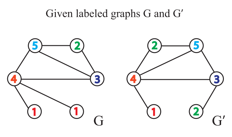
Weisfeiler Leman test algorithm judges whether the graph is isomorphic by repeating the following process of labeling nodes:
-
Aggregate the labels of itself and adjacent nodes to obtain a string. The labels of itself and adjacent nodes are separated by, and the labels of adjacent nodes are sorted in ascending order. The reason for sorting is to ensure the injectivity, that is, to ensure that the obtained results do not change due to the change of the order of adjacent nodes
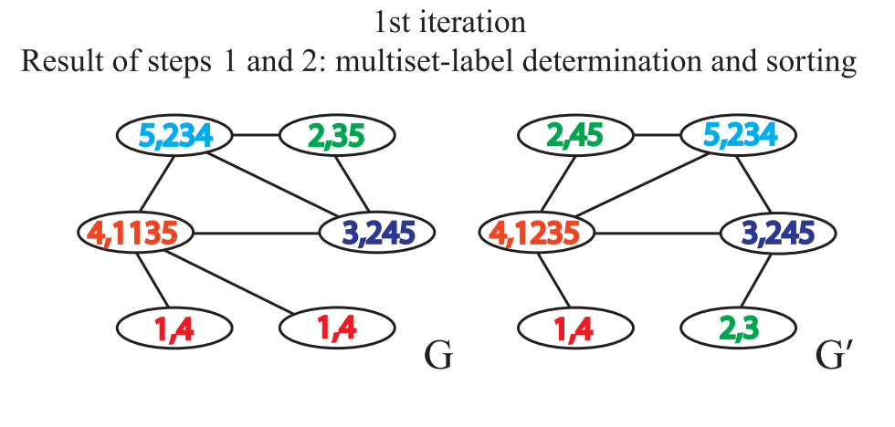
-
Tag hashing, or tag compression, maps a longer string to a shorter tag
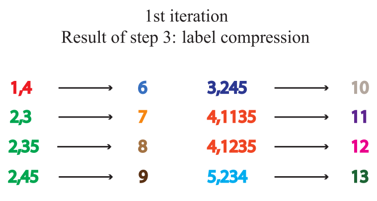
-
Relabel nodes
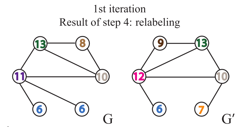
Each time the process is repeated more than once, the aggregation of node labels and adjacent node labels is completed
When the occurrence times of the same node labels of two graphs are inconsistent, it can be judged that the two graphs are not similar. If the above steps are repeated for a certain number of times and there is no inconsistency in the number of occurrences of the same node label, we cannot judge whether the two graphs are isomorphic
Figure similarity assessment
One limitation of WL Test algorithm is that it can only judge the similarity of two graphs, and can not measure the similarity between graphs. To measure the similarity between the two graphs, we use the WL Subtree Kernel method. The idea of this method is to use WL Test algorithm to obtain multi-layer labels of nodes, and then we can count the times of various labels in the graph and store them in a vector, which can be used as the representation of the graph. The inner product of such a vector of two graphs can be used as an estimate of the similarity of the two graphs
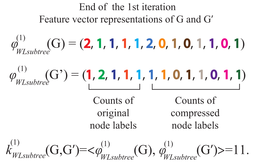
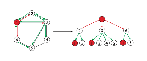
WL subtree
When two nodes h h When the labels of layer h are the same, it means that the WL subtrees with these two nodes as root nodes are consistent. WL subtree is different from ordinary subtree. WL subtree contains duplicate nodes. The following figure shows a WL subtree with node 1 as the root and node height 2
Construction of graph isomorphic network model
The graph neural network that can judge graph isomorphism needs to meet the following requirements. Only when the labels of two nodes are the same and their adjacent nodes are the same, the graph neural network maps the two nodes to the same representation, that is, the mapping is injective. Repeatable sets refer to sets in which elements can be repeated, and elements have no sequential relationship in the set** All adjacent nodes of a node are a repeatable set. A node can have duplicate adjacent nodes, and the adjacent nodes have no sequential relationship** Therefore, the method of generating node representation in GIN model follows the process of updating node label by WL Test algorithm.
After generating the representation of nodes, it is still necessary to perform graph pooling (or graph readout) to obtain graph features. The simplest graph readout operation is summation. Since the node representation of each layer may be important, in a graph isomorphic network, the node representations of different layers are spliced after summation. Its mathematical definition is as follows,
h
G
=
CONCAT
(
READOUT
(
{
h
v
(
k
)
∣
v
∈
G
}
)
∣
k
=
0
,
1
,
⋯
,
K
)
h_{G} = \text{CONCAT}(\text{READOUT}\left(\{h_{v}^{(k)}|v\in G\}\right)|k=0,1,\cdots, K)
hG=CONCAT(READOUT({hv(k)∣v∈G})∣k=0,1,⋯,K)
* * the reason for using splicing rather than addition is that the representation of nodes in different layers belongs to different feature spaces** Without strict proof, the representation of the graph obtained in this way is equivalent to the representation of the graph obtained by WL Subtree Kernel
task
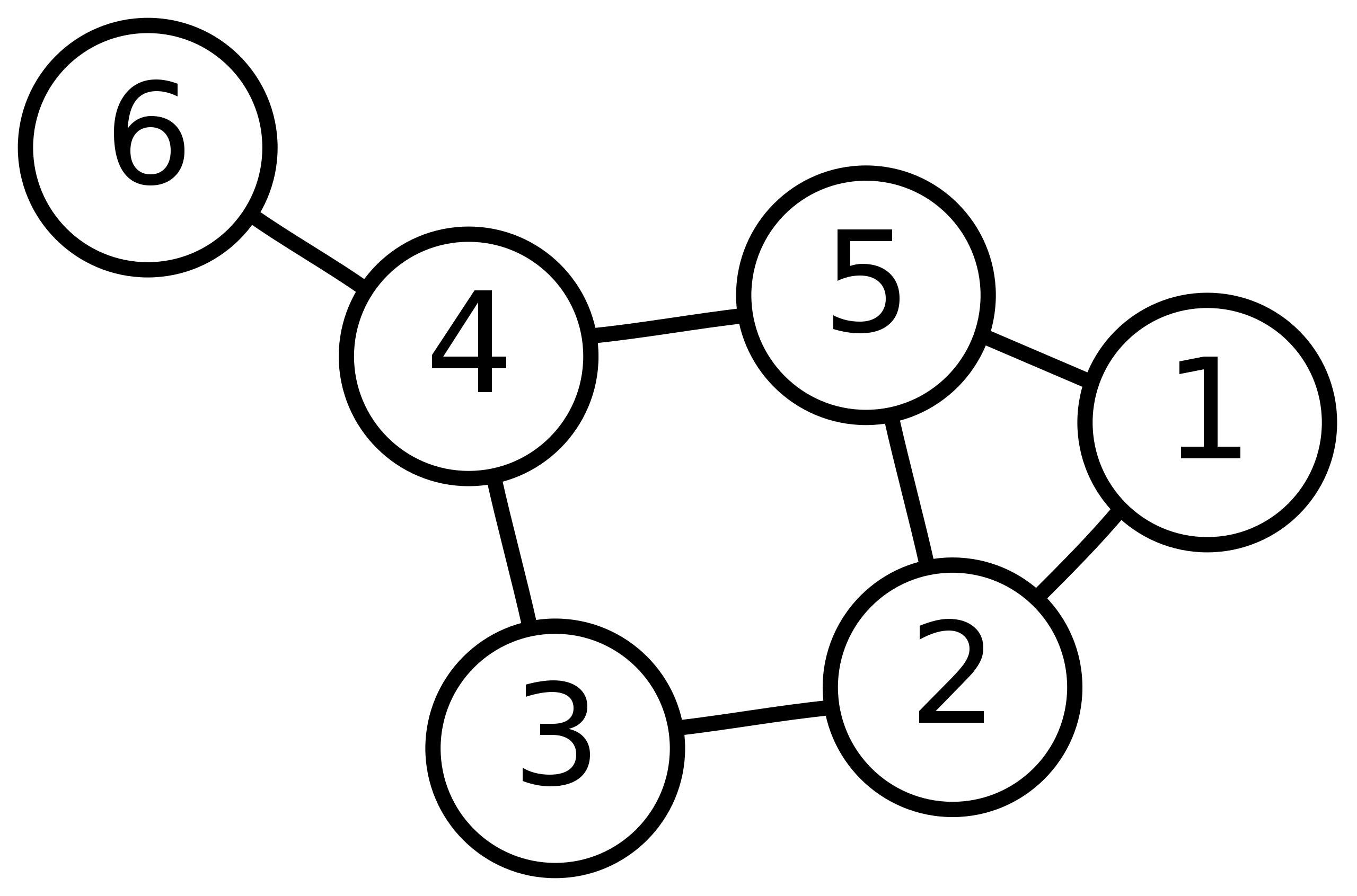
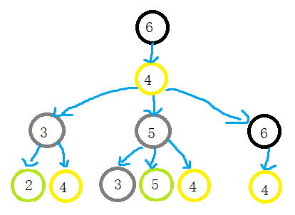
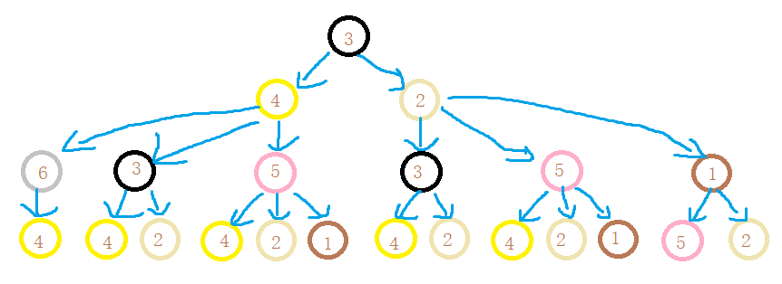
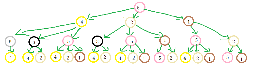
-
Please draw the WL subtree from layer 1 to layer 3 of nodes 6, 3 and 5 in the picture below.