Tweet before Detailed explanation of python scipy sparse matrix The principle of common sparse matrix and its application experience in python are introduced in detail. This tweet focuses on R language sparse matrix format and its application in single cell multiomics (scRNA, scATAC).
R sparse matrix
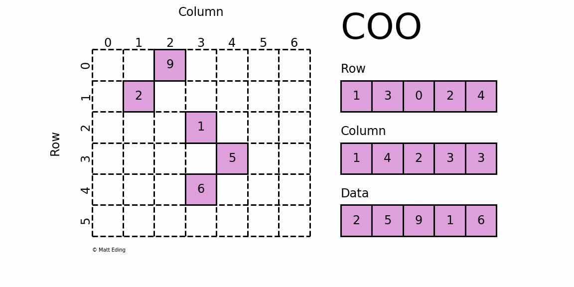
dgTMatrix
That is, Sparse matrices in triplet form, which is similar to coo in python_ Matrix is the simplest storage method of sparse matrix. It uses the form of triple (row, col, data) (or ijv format) to store the information of non-zero elements in the matrix.
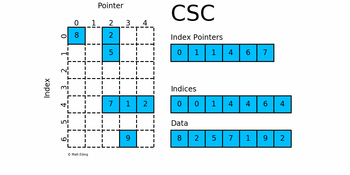
dgCMatrix
Compressed, sparse, column oriented numeric matrices, which is similar to CSC in Python_ Matrix is a sparse matrix format compressed by column, which is composed of three one-dimensional arrays indptr, indices and data. dgCMatrxi is the standard format and the most common format in R-Pack matrix. This format is generally used for sparse data storage of single cell multiomics.
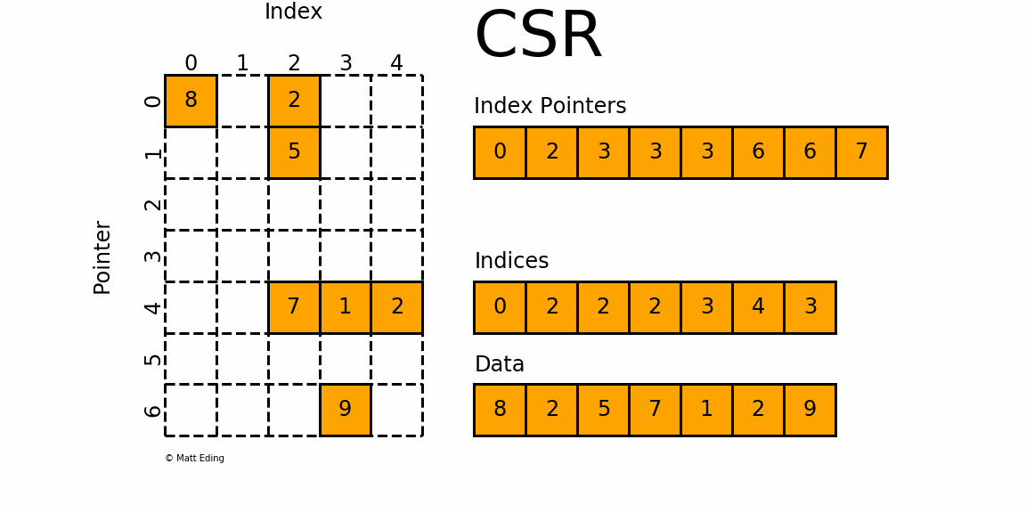
dgRMatrix
That is, sparse compressed, row oriented numeric matrices, which is similar to CSR in Python_ Matrix, contrary to dgCMatrxi, the sparse matrix of this format is compressed by rows. In principle, it is also composed of three one-dimensional arrays indptr, indices and data. dgRMatrxi sparse matrix is generally not used in single-cell omics analysis. The implementation of rmdxi is similar to that of rmdxi.
Common operation methods of R sparse matrix
Sparse matrix construction
######dgCMatrix######
Method 1: Matrix(*, sparse = TRUE)
#Matrix package
mat <- Matrix(data = 0L, nrow=3201, ncol = 818, sparse = TRUE) #dgCMatrix
print(object.size(mat), unit="KB")
#4.7 Kb
dim(mat)
#[1] 3201  818

Method 2: sparseMatrix()
#Matrix package
i <- c(1,3:8)
j <- c(2,9,6:10)
x <- 7 * (1:7)
mat2 <- sparseMatrix(i, j, x = x) # dgCMatrix

Method 3: as(*, "dgCMatrix")
mat3 <- matrix(data=c(0,0,1,2,0,3,0,0,0), nrow=3, ncol=3) #Matrix built-in function, which is used to build a general matrix.
mat3 <- as(mat3, "dgCMatrix") # dgCMatrix
#3 x 3 sparse Matrix of class "dgCMatrix"
#[1,] . 2 .
#[2,] . . .
#[3,] 1 3 .

Method 4: new("dgCMatrix", ...),...Fill in at dgCMatrix Class
#Although R is a statistical language, R can also be object-oriented programming. S4 object is a standard object-oriented implementation, with special class definition function setClass() and class instantiation function new(). "dgCMatrix" is essentially a class, so we can directly instantiate this class with the new function to create objects.
indptr <-  c(2L, 0L, 2L) #Must be an integer
indices <- c(0L, 1L, 3L, 3L) #Must be an integer
data <- c(1, 2, 3)
mat4 <- new('dgCMatrix', i=indptr, p=indices, x=data, Dim=c(3L,3L))  #The Dim parameter must be an integer


######dgTMatrix######
Method 1: sparseMatrix()
#Matrix package
i <- c(1,3:8)
j <- c(2,9,6:10)
x <- 7 * (1:7)
mat1 <- sparseMatrix(i, j, x = x, repr = "T")

Method 2: spMatrix()
#Matrix package
mat2 <- spMatrix(10,20, i = c(1,3:8),
                     j = c(2,9,6:10),
                     x = 7 * (1:7))

Method 3: as(*, "dgTMatrix") #It's the same as building dgC matrix, so I won't repeat it

Method 4: new("dgTMatrix", ...) #It's the same as building dgC matrix, so I won't repeat it
Sparse matrix format conversion
#dense matrix to sparse matrix
sparse_matrix <- as(dense_matrix, "dgCMatrix")
sparse_matrix <- as(dense_matrix, "dgTMatrix")
sparse_matrix <- as(dense_matrix, 'sparseMatrix')  # dgCMatrix
sparse_matrix <- as(dense_matrix, 'Matrix')  # dgCMatrix

#sparse matrix to dense matrix
dense_matrix <- as.matrix(sparse_matrix)
dense_matrix <- as(sparse_matrix, 'matrix')

#dgCMatrix to dgTMatrix
dgC_matrix <- as(dgT_matrix, 'dgCMatrix')
dgT_matrix <- as(dgC_matrix, 'dgTMatrix')
In fact, there is an R package SparseM Package can easily operate sparse matrix. The name of sparse matrix in this R package is the same as that in python, that is, csc, csr and coo sparse matrix. Interested readers can understand it by themselves.
Sparse matrix judgment
Sometimes it is necessary to judge whether the matrix is sparse and what kind of sparse matrix it is. You can use the following command:
i <- c(1,3:8)
j <- c(2,9,6:10)
x <- 7 * (1:7)
mat <- sparseMatrix(i, j, x = x, repr = "T") # Create dgTMatrix
is(mat, 'sparseMatrix')
#[1] TRUE
is(mat, 'dgTMatrix')
#[1] TRUE
is(mat, 'dgCMatrix')
#[1] FALSE
is(mat, 'Matrix')
#[1] TRUE
is(mat, 'matrix') #It should be noted that the matrix package is usually used to operate sparse matrices, while the built-in function matrix is used to operate conventional matrices.
#[1] FALSE
Sparse matrix reading and writing
#Generally, the reading and saving of sparse Matrix is realized through Matrix package.
Matrix::readMM #Read sparse matrix
Matrix::writeMM #Save sparse matrix
Application of sparse matrix in single cell multiomics
Cellranger
The following is the result generated by Cellranger, where matrix MTX files are in dgTMatrix format, so if the downstream analysis software requires sparse matrices in other formats, conversion steps are required.
$ tree filtered_feature_bc_matrix/
filtered_feature_bc_matrix/
├── barcodes.tsv.gz
├── features.tsv.gz
└── matrix.mtx.gz  dgT format
Seurat
One big difference between using Seurat and Scanpy to analyze single-cell data is that each behavior in the Annadata object is one cell, while the Seurat object is the opposite. dgCMatrix is used for single cell sparse data storage in Seurat; The sparse storage mode of Cellranger output to file is dgTMatrix format, so it is necessary to convert the sparse matrix format before analyzing the data output by Cellranger with Seurat. This is the core implementation of Seurat::Read10X function, which will generate dgCMatrix with row and column names. Of course, you can also use this function to build a sparse matrix by yourself, and then use the CreateSeuratObject function to generate Seurat objects. Reference codes are as follows:
## construct RNA Seurat object
dir.10x = './filtered_feature_bc_matrix'
genes = read.delim(paste0(dir.10x, 'genes.tsv'), row.names = 1)
barcodes = read.delim(paste0(dir.10x, 'barcodes.tsv'), row.names = 1)
mtx = Matrix::readMM(paste0(dir.10x, 'matrix.mtx'))
mtx = as.matrix(mtx)
mtx = as(mtx, 'dgCMatrix') #Convert the sparse matrix to Seurat's default dgC format
colnames(mtx) = row.names(barcodes)
rownames(mtx) = row.names(genes)
pbmc = CreateSeuratObject(counts = mtx, assay = 'RNA', meta.data = barcodes)
Signac
For the import of Cellranger data, you can use Seurat::Read10X and Seurat::Read10X_h5 function. However, when we download data from a public database, in many cases, we can only download three files generated by cell Ranger ATAC: barcodes tsv,matrix.mtx and peaks bed. In this case, we can either forcibly try the Seurat::Read10X function or implement a reading method ourselves.
If you directly use Seurat::Read10X to read these three files, you will find an error in the code for two reasons:
- The file name is incorrect. Because the three file names read in by Seurat::Read10X by default are barcodes tsv. gz,features.tsv.gz and matrix mtx. GZ, while the file names output by cell Ranger ATAC are different.
- The Seurat::Read10X function needs to read non duplicate barcodes and features(gene name or peak ID), but peaks Bed does not provide a unique peak ID.
Therefore, method 1, modify peaks The bed file content, and then read it using the Seurat::Read10X function
# peaks. The bed file format does not have a unique peak ID, so it needs to be converted.
chr1	9757	10652
chr1	86735	87645
chr1	180601	181169
#To peaks Add peak ID to bed file, and the construction method is the same as above; Then modify the file name; Finally, read with Read10X function.
data.dir <- './filtered_peak_bc_matrix'
features <- read.csv('./filtered_peak_bc_matrix/peaks.bed',  header = FALSE, row.names = NULL, sep = '\t')
row.names(features) <- paste(paste(features$V1, features$V2, sep=':'), features$V3, sep='-')   #Build peak ID
features <- features['V1']  #Take out the peak ID column separately and save it
write.table(features, './filtered_peak_bc_matrix/features.tsv', sep = '\t', row.names=F, col.names=F, quote = F)
#Next, modify other file names, that is, they can be read by the Read10X function.
counts <- Read10X(data.dir,gene.column = 1, cell.column = 1)
chrom_assay <- CreateChromatinAssay(counts = counts,
                                    sep = c(":", "-"), genome = 'hg19',
  																	# fragments = '../vignette_data/atac_v1_pbmc_10k_fragments.tsv.gz', #You can't provide this file without it, so you can't draw a track diagram later
  																	min.cells = 10,
  																	min.features = 200)
pbmc <- CreateSeuratObject(counts = chrom_assay, assay = "peaks")
Method 2: read the data by yourself and build the object
#Read10X_ The h5 function essentially generates a dgCMatrix with row and column names, so if we don't have an h5 file, we can directly build this matrix ourselves.
dir.10x = './filtered_feature_bc_matrix'
features = read.csv(paste0(dir.10x, 'peaks.bed'), header = FALSE, row.names = NULL, sep = '\t')
row.names(features) <- paste(paste(features$V1, features$V2, sep=':'), features$V3, sep='-')  #Build peak ID
barcodes = read.delim(paste0(dir.10x, 'barcodes.tsv'), row.names = 1)
mtx = Matrix::readMM(paste0(dir.10x, 'matrix.mtx'))
colnames(mtx) = row.names(barcodes)
mtx = as(mtx, 'dgCMatrix') #The sparse matrix generated here is equivalent to Read10X_h5 generated sparse matrix, use this object to continue downstream analysis.
chrom_assay <- CreateChromatinAssay(counts = mtx,
                                    sep = c(":", "-"), genome = 'hg19',
  																	# fragments = '../vignette_data/atac_v1_pbmc_10k_fragments.tsv.gz', #If there is no such file, it can not be provided, so the fragments related analysis cannot be performed later
  																	min.cells = 10,
  																	min.features = 200)
pbmc <- CreateSeuratObject(counts = chrom_assay, assay = "peaks")
reference material
Official account - programming study room: sparse matrix analysis and single cell data reading