This note is based on the tensorflow-2 version and is contributed first code perhaps Download code (scientific Internet access may be required).

What is image segmentation

In the image classification task, the network assigns a label (or category) to each input image. However, suppose you want to know the shape of the object, which pixel belongs to which object, and so on. In this case, you want to assign a category to each pixel of the image. This task is called segmentation. A segmentation model returns more detailed information about the image. Image segmentation has many applications in medical imaging, autopilot and satellite imaging, for example.

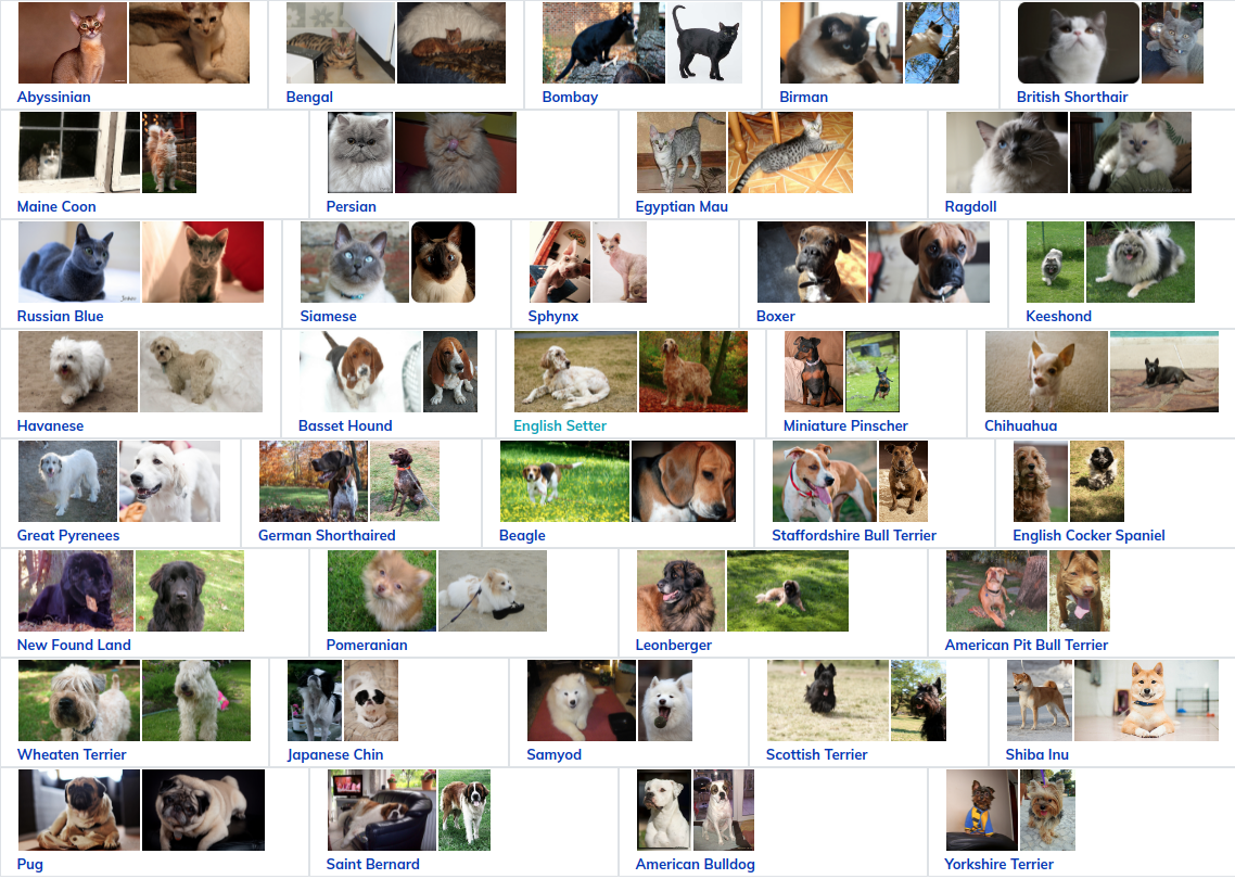
Here's one data set , the data set consists of images of 37 pet breeds, each with 200 images (about 100 in the training and testing parts). Each picture includes a corresponding label and pixel level mask. The mask is the category label for each pixel. Each pixel is assigned to one of three categories:

• Category I: pixels representing pets
• Category II: pixels bordering the edge of pets
• Category 3: none of the above pixels
  The example can be installed through the following program:

pip install git+https://github.com/tensorflow/examples.git

If the GitHub cannot be linked or the connection speed is slow, you can install it through this image. Similarly, any other GitHub package can be downloaded or installed using this image:

pip install git+https://github.com.cnpmjs.org/tensorflow/examples.git

Import TensorFlow related packages:

import tensorflow as tf
from tensorflow.keras.layers.experimental import preprocessing 

import tensorflow_datasets as tfds

from tensorflow_examples.models.pix2pix import pix2pix

from IPython.display import clear_output
import matplotlib.pyplot as plt

Download Oxford IIIT PET data (download size 773.52M, dataset size 774.69M):

dataset, info = tfds.load('oxford_iiit_pet:3.*.*', with_info=True)

it's fine too Manual Download.
Picture display:

In addition, the image color values are normalized to the [0,1] range. Finally, as described above, the pixels in the segmentation are marked as {1, 2, 3}. For convenience, subtract 1 from the tag to get the tag: {0, 1, 2}:

def normalize(input_image, input_mask):
  input_image = tf.cast(input_image, tf.float32) / 255.0
  input_mask -= 1
  return input_image, input_mask

arrangement:

def load_image(datapoint):
  input_image = tf.image.resize(datapoint['image'], (128, 128))
  input_mask = tf.image.resize(datapoint['segmentation_mask'], (128, 128))

  input_image, input_mask = normalize(input_image, input_mask)

  return input_image, input_mask

The data set has been divided into test set and training set, so it does not need to be subdivided and can be used directly:

TRAIN_LENGTH = info.splits['train'].num_examples
BATCH_SIZE = 64
BUFFER_SIZE = 1000
STEPS_PER_EPOCH = TRAIN_LENGTH // BATCH_SIZE

The following class performs a simple amplification, that is, randomly flipping an image:

class Augment(tf.keras.layers.Layer):
  def __init__(self, seed=42):
    super().__init__()
    # both use the same seed, so they'll make the same randomn changes.
    self.augment_inputs = preprocessing.RandomFlip(mode="horizontal", seed=seed)
    self.augment_labels = preprocessing.RandomFlip(mode="horizontal", seed=seed)

  def call(self, inputs, labels):
    inputs = self.augment_inputs(inputs)
    labels = self.augment_labels(labels)
    return inputs, labels

Build the input pipeline, batch process the input, and then use the Augmentation:

train_batches = (
    train_images
    .cache()
    .shuffle(BUFFER_SIZE)
    .batch(BATCH_SIZE)
    .repeat()
    .map(Augment())
    .prefetch(buffer_size=tf.data.AUTOTUNE))

test_batches = test_images.batch(BATCH_SIZE)

Image example and its MASK diagram:

def display(display_list):
  plt.figure(figsize=(15, 15))

  title = ['Input Image', 'True Mask', 'Predicted Mask']

  for i in range(len(display_list)):
    plt.subplot(1, len(display_list), i+1)
    plt.title(title[i])
    plt.imshow(tf.keras.preprocessing.image.array_to_img(display_list[i]))
    plt.axis('off')
  plt.show()
for images, masks in train_batches.take(2):
  sample_image, sample_mask = images[0], masks[0]
  display([sample_image, sample_mask])

The Unet model is defined below

We use the improved unet network model here. A unet consists of an encoder (lower sampler) and a decoder (upper sampler). In order to learn image features more robustly and reduce the number of trainable parameters, a pre trained model MobileNetV2 will be used as the encoder. For the decoder, you can use the up sampling module, which has been implemented in Pix2pix in TensorFlow instance library.

The encoder is a trained MobileNetV2 model. You can directly call tf.keras.applications. The encoder is composed of the specific output of the middle layer of the model, and the encoder will not be trained in the training process.

base_model = tf.keras.applications.MobileNetV2(input_shape=[128, 128, 3], include_top=False)

# Use the activations of these layers
layer_names = [
    'block_1_expand_relu',   # 64x64
    'block_3_expand_relu',   # 32x32
    'block_6_expand_relu',   # 16x16
    'block_13_expand_relu',  # 8x8
    'block_16_project',      # 4x4
]
base_model_outputs = [base_model.get_layer(name).output for name in layer_names]

# Create the feature extraction model
down_stack = tf.keras.Model(inputs=base_model.input, outputs=base_model_outputs)

down_stack.trainable = False

Decoder / upsampling is only a series of upsampling modules implemented in TensorFlow.

up_stack = [
    pix2pix.upsample(512, 3),  # 4x4 -> 8x8
    pix2pix.upsample(256, 3),  # 8x8 -> 16x16
    pix2pix.upsample(128, 3),  # 16x16 -> 32x32
    pix2pix.upsample(64, 3),   # 32x32 -> 64x64
]

def unet_model(output_channels:int):
  inputs = tf.keras.layers.Input(shape=[128, 128, 3])

  # Downsampling through the model
  skips = down_stack(inputs)
  x = skips[-1]
  skips = reversed(skips[:-1])

  # Upsampling and establishing the skip connections
  for up, skip in zip(up_stack, skips):
    x = up(x)
    concat = tf.keras.layers.Concatenate()
    x = concat([x, skip])

  # This is the last layer of the model
  last = tf.keras.layers.Conv2DTranspose(
      filters=output_channels, kernel_size=3, strides=2,
      padding='same')  #64x64 -> 128x128

  x = last(x)

  return tf.keras.Model(inputs=inputs, outputs=x)

Note: the number of filters on the previous layer is set to the number of output channels, which is also the number of output channels of this layer.

Training model

This is a multi classification problem. Cetegfornicalcrossentropy (from_logits=True) is used as the standard loss function, that is, losses.SparseCategoricalCrossentropy(from_logits=True) is used because the label is scalar rather than the fractional vector of each class.

OUTPUT_CLASSES = 3

model = unet_model(output_channels=OUTPUT_CLASSES)
model.compile(optimizer='adam',
              loss=tf.keras.losses.SparseCategoricalCrossentropy(from_logits=True),
              metrics=['accuracy'])

Model detection:

tf.keras.utils.plot_model(model, show_shapes=True)

Test the model before training:

def create_mask(pred_mask):
  pred_mask = tf.argmax(pred_mask, axis=-1)
  pred_mask = pred_mask[..., tf.newaxis]
  return pred_mask[0]

def show_predictions(dataset=None, num=1):
  if dataset:
    for image, mask in dataset.take(num):
      pred_mask = model.predict(image)
      display([image[0], mask[0], create_mask(pred_mask)])
  else:
    display([sample_image, sample_mask,
             create_mask(model.predict(sample_image[tf.newaxis, ...]))])

Output:

show_predictions()

Feedback is defined below to improve accuracy during training:

class DisplayCallback(tf.keras.callbacks.Callback):
  def on_epoch_end(self, epoch, logs=None):
    clear_output(wait=True)
    show_predictions()
    print ('\nSample Prediction after epoch {}\n'.format(epoch+1))

EPOCHS = 20
VAL_SUBSPLITS = 5
VALIDATION_STEPS = info.splits['test'].num_examples//BATCH_SIZE//VAL_SUBSPLITS

model_history = model.fit(train_batches, epochs=EPOCHS,
                          steps_per_epoch=STEPS_PER_EPOCH,
                          validation_steps=VALIDATION_STEPS,
                          validation_data=test_batches,
                          callbacks=[DisplayCallback()])

Loss function:

loss = model_history.history['loss']
val_loss = model_history.history['val_loss']

plt.figure()
plt.plot(model_history.epoch, loss, 'r', label='Training loss')
plt.plot(model_history.epoch, val_loss, 'bo', label='Validation loss')
plt.title('Training and Validation Loss')
plt.xlabel('Epoch')
plt.ylabel('Loss Value')
plt.ylim([0, 1])
plt.legend()
plt.show()

forecast:

show_predictions(test_batches, 3)

Semantic segmentation data sets may be highly unbalanced, which means that pixels of a specific category can have higher weights than other pixels. Since the segmentation problem can be handled by pixel level problem, we can deal with the imbalance problem by weighted loss function. Can refer to here.
model.fit does not support 3 + dimension data at present:

try:
  model_history = model.fit(train_batches, epochs=EPOCHS,
                            steps_per_epoch=STEPS_PER_EPOCH,
                            class_weight = {0:2.0, 1:2.0, 2:1.0})
  assert False
except Exception as e:
  print(f"{type(e).__name__}: {e}")

report errors:

ValueError: `class_weight` not supported for 3+ dimensional targets.

Therefore, we need to implement weighting ourselves. You can refer to the sample weight: model.fit can accept (data, label) format and (data, label, sample_weight) 3D style.

model.fit can convert sample_weight is passed to the loss function and matrix, and then the sample weight is multiplied by the sample. For example:

label = [0,0]
prediction = [[-3., 0], [-3, 0]] 
sample_weight = [1, 10] 

loss = tf.losses.SparseCategoricalCrossentropy(from_logits=True,
                                               reduction=tf.losses.Reduction.NONE)
loss(label, prediction, sample_weight).numpy()

Therefore, in order to generate the sample weight, we need a function, which inputs (data, label) and then outputs (data, label, sample_weight). The sample weight includes the weight of each pixel.

The simplest is to use the label as the index of the weight list:

def add_sample_weights(image, label):
  # The weights for each class, with the constraint that:
  #     sum(class_weights) == 1.0
  class_weights = tf.constant([2.0, 2.0, 1.0])
  class_weights = class_weights/tf.reduce_sum(class_weights)

  # Create an image of `sample_weights` by using the label at each pixel as an 
  # index into the `class weights` .
  sample_weights = tf.gather(class_weights, indices=tf.cast(label, tf.int32))

  return image, label, sample_weights

Each component of the generated dataset contains three elements:

train_batches.map(add_sample_weights).element_spec

Now we can train the model on the weighted data set:

weighted_model = unet_model(OUTPUT_CLASSES)
weighted_model.compile(
    optimizer='adam',
    loss=tf.keras.losses.SparseCategoricalCrossentropy(from_logits=True),
    metrics=['accuracy'])

weighted_model.fit(
    train_batches.map(add_sample_weights),
    epochs=1,
    steps_per_epoch=10)