Histogram equalization

Let's take a look at the renderings:

digital image

I think everyone should have some concepts about the concept of digital image. In the past, photos were exposed by camera using film. The photosensitive material on the film will form an exposure point when light shines on it. After an image is mapped in, a picture is formed in the negative. After getting the film, we need to go through special processing (film development) to get my picture.
But now the images are stored in memory after digital processing, which are digital images. For example, binary images, 1 represents black and 0 represents white, which are stored in memory in the form of a two-dimensional matrix. The color image is a little more complex (the color image we are talking about now is RGB image). I put the storage form of RGB image in my first blog:
Image interpolation algorithm for RGB and other pictures is implemented in pure python
In this link, the feeling is still relatively clear. There are some pictures that can help understand three-dimensional RGB images.

What is the histogram in the image?

Histogram of digital image. Histogram is the basis of multi spatial domain processing technology. Histogram operation can act on image enhancement. The theorem in the book is more formal and needs to be understood by yourself. Here is my own understanding. First, I quote the original text of Gonzalez's digital image processing:

In fact, it is the histogram statistics in mathematics. The image (single channel) read out by the array is actually a two-dimensional array. Each number in the two-dimensional array is a gray level (the larger the gray level, the greater the brightness, and the range is 0 ~ 255, 8bit image).
Please look at the following picture:

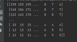
The number inside is the result of reading a picture (channel 0 of a color picture). The number inside is between 0 and 255. Well, we now have this concept.
Next, we will make statistics on each gray level inside. For example, we need to make statistics on gray level 12, count how many 12 gray levels appear in this array, and draw the number corresponding to different gray levels back into a statistical histogram, which is the histogram of the picture.
Let's take a look at how to make probability statistics on the data in a picture, and directly look at the core code:

hist = defaultdict(lambda: 0)  # Define a dictionary to store the number of gray levels after statistics
        for i in range(size_h):
            for j in range(size_w):
                hist[img[i, j]] += 1

We traverse each pixel of the image and store it in the hist dictionary after statistics. The key in the dictionary is the gray level of 0 ~ 255.

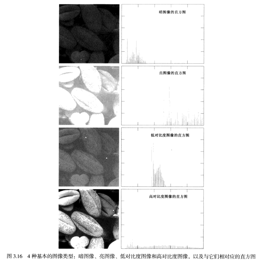
Let's take a look at what a digital image without histogram equalization looks like. Here I still quote what Gonzalez said in digital image processing:

normalization

Using probability distribution, for this image sample, the probability of gray level 12 is the statistical number we just calculated divided by all sample points (M*N). All gray levels in the whole picture are statistically calculated, so that we can get the probability statistics of each gray level, and then draw all the probability statistics into a square statistical diagram to get the histogram of the digital image (normalized histogram).
Normalization is to divide these statistical data by 256. Because there are 256 gray levels, the data is normalized after dividing by 256, which is the normalization of the histogram.

Histogram equalization

continuity

dispersed

Discrete transformation form, which is also the formula we will use next.

The equalization code is given below, where the parameter color_pic=True means that what we send in is a color picture, and the gray-scale picture can also be equalized.

       def equalize_histogram_pic(img, color_pic=True):
        """Histogram equalization"""
        hist = Histogram.get_histogram(img, color_pic=color_pic)  # Get the picture transmitted from the instantiated object and get its histogram
        size_h, size_w= img.shape[0], img.shape[1]
        MN = size_h * size_w  # Get M*N

        new_gray_level = defaultdict(lambda: 0)  # Define a dictionary to store the equalization transformation mapping of gray level
        print("we are equalizing...")
        for i in range(256):
            for key in range(i + 1):
                new_gray_level[i] += hist[key]  # Add the first i gray level values to the i gray level
            new_gray_level[i] = new_gray_level[i] * 255 / MN  # Take out the number of the ith gray level and multiply it by 255/MN to save the mapping result of Sk in the dictionary, which is the discrete calculation formula of Sk in the book
            new_gray_level[i] = round(new_gray_level[i])  # The gray value is rounded for equalization mapping

        # The new gray mapping relationship is mapped from the original image to the equalized image
        new_img = img.copy()  # Copy the original image, and then update the gray value mapping relationship in the new image
        for i in range(new_img.shape[0]):
            for j in range(new_img.shape[1]):
                new_img[i, j] = new_gray_level[new_img[i, j, 0]]  # The new gray mapping relationship is mapped from the original image to the equalized image
        print('The equalizing ok')
        return new_img

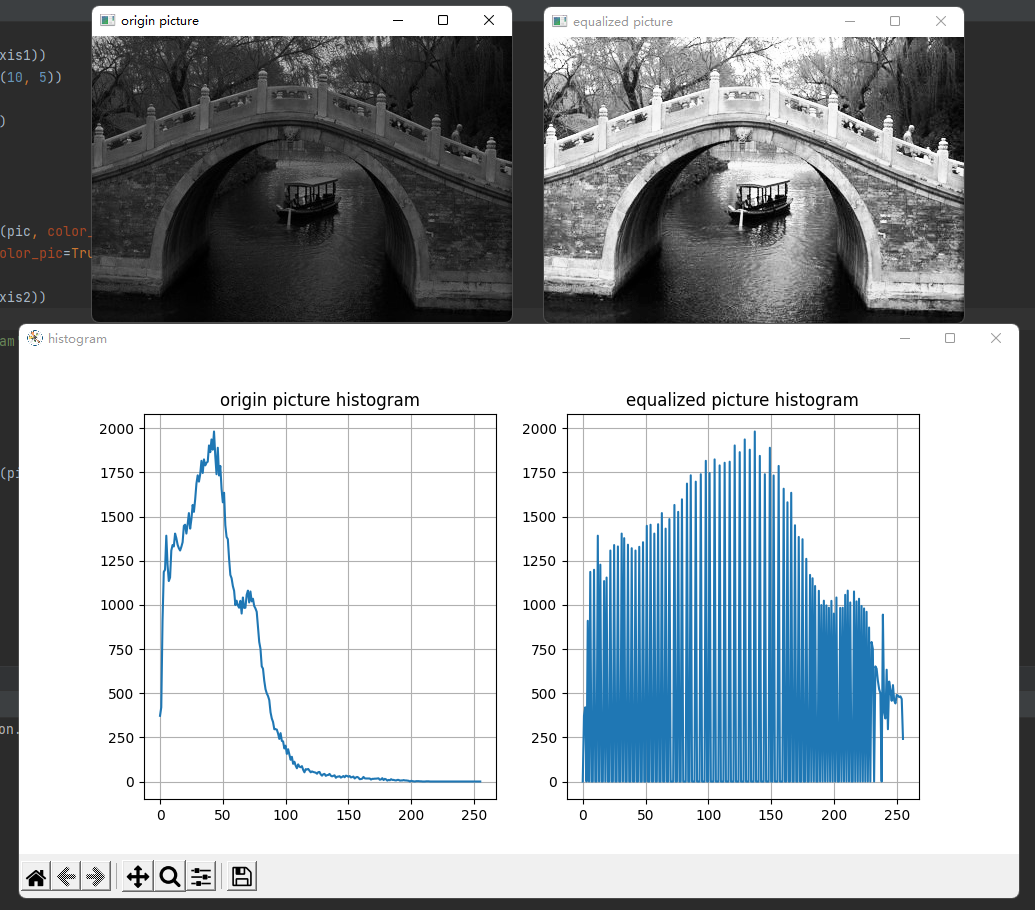
Here are the results after equalization:

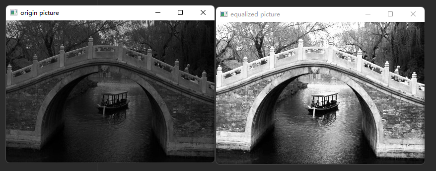
After the darker part of the original picture is balanced, we look clearer. Let's look at their histogram.
Let's see how to get the statistical picture from the dictionary. Look at the following code:

 pic = cv2.imread(r'./bridge.jpg')
    hist1 = Histogram.get_histogram(pic, color_pic=True)
    x_axis1 = range(0, 256)
    y_axis1 = list(map(lambda i: hist1[i], x_axis1))
    fig = plt.figure(num='histogram', figsize=(10, 5))
    plot1 = fig.add_subplot(121)
    plot1.set_title('origin picture histogram')
    plot1.plot(x_axis1, y_axis1)
    plot1.grid()

enclosure

All my codes are attached below:

import matplotlib.pyplot as plt
import numpy as np
from collections import defaultdict
import cv2
import logging


class Histogram(object):
    def __int__(self):
        pass

    def get_histogram(img_x, *, color_pic=True, normalized=False):
        if color_pic:             # color_pic is used to specify a color picture
            img = img_x[:, :, 0]  # Only channel 0 of the color image is taken out
        else:
            img = img_x
        size_h, size_w = img.shape
        logging.info(fr'size_h: {size_h}, size_w: {size_w}')
        print(fr'size_h: {size_h}, size_w: {size_w}')
        hist = defaultdict(lambda: 0)  # Define a dictionary to store the number of gray levels after statistics
        for i in range(size_h):
            for j in range(size_w):
                hist[img[i, j]] += 1

        # Decide whether to normalize according to the normalized parameter
        if normalized:
            sum = 0
            MN = size_h * size_w
            for key in hist:
                hist[key] = hist[key] / MN
                sum += hist[key]
            logging.info(f'The normalized value is:{sum},Normalized statistical value:{hist}')
            print('Normalized sum:', sum)
            del sum
            logging.info(f'Statistical value:{hist}')

        return hist

    # @staticmethod
    def equalize_histogram_pic(img, color_pic=True):   # color_pic is used to specify a color picture
        """Histogram equalization"""
        hist = Histogram.get_histogram(img, color_pic=color_pic)  # Get the picture transmitted from the instantiated object and get its histogram
        size_h, size_w= img.shape[0], img.shape[1]
        MN = size_h * size_w  # Get M*N

        new_gray_level = defaultdict(lambda: 0)  # Define a dictionary to store the equalization transformation mapping of gray level
        print("we are equalizing...")
        for i in range(256):
            for key in range(i + 1):
                new_gray_level[i] += hist[key]  # Add the first i gray level values to the i gray level
            new_gray_level[i] = new_gray_level[i] * 255 / MN  # Take out the number of the ith gray level and multiply it by 255/MN to save the mapping result of Sk in the dictionary, which is the discrete calculation formula of Sk in the book
            new_gray_level[i] = round(new_gray_level[i])  # The gray value is rounded for equalization mapping

        # The new gray mapping relationship is mapped from the original image to the equalized image
        new_img = img.copy()  # Copy the original image, and then update the gray value mapping relationship in the new image
        for i in range(new_img.shape[0]):
            for j in range(new_img.shape[1]):
                new_img[i, j] = new_gray_level[new_img[i, j, 0]]  # The new gray mapping relationship is mapped from the original image to the equalized image
        print('The equalizing ok')
        return new_img

if __name__ == '__main__':
    pic = cv2.imread(r'./bridge.jpg')
    hist1 = Histogram.get_histogram(pic, color_pic=True)
    x_axis1 = range(0, 256)
    y_axis1 = list(map(lambda i: hist1[i], x_axis1))
    fig = plt.figure(num='histogram', figsize=(10, 5))
    plot1 = fig.add_subplot(121)
    plot1.set_title('origin picture histogram')
    plot1.plot(x_axis1, y_axis1)
    plot1.grid()

    # new_ Histogram of PIC
    new_pic = Histogram.equalize_histogram_pic(pic, color_pic=True)
    hist2 = Histogram.get_histogram(new_pic, color_pic=True)
    x_axis2 = range(0, 256)
    y_axis2 = list(map(lambda i: hist2[i], x_axis2))
    plot2 = fig.add_subplot(122)
    plot2.set_title('equalized picture histogram')
    plot2.plot(x_axis2, y_axis2)
    plot2.grid()

    # Equalization
    # cv2.imshow('origin picture', pic)
    # new_pic = Histogram.equalize_histogram_pic(pic, color_pic=True)
    # print(new_pic.shape)
    # cv2.imshow('equalized picture', new_pic)

    plt.show()