MNIST dataset
MNIST dataset is already a "chewed" dataset. Many tutorials will "start" on it and almost become a "model" However, some people may not know it very well. Let's introduce it
MNIST datasets are available in http://yann.lecun.com/exdb/mnist/ Get, which consists of four parts:
Training set images: train-images-idx3-ubyte.gz (9.9 MB, 47 MB after decompression, including 60000 samples)
Training set labels: train-labels-idx1-ubyte.gz (29 KB, 60 KB after decompression, including 60000 tags)
Test set images: t10k-images-idx3-ubyte.gz (1.6 MB, 7.8 MB after decompression, including 10000 samples)
Test set labels: t10k-labels-idx1-ubyte.gz (5KB, 10KB after decompression, including 10000 tags)
MNIST data set is from National Institute of Standards and Technology (NIST) The training set consists of 250 handwritten numbers from different people, of which 50% are high school students and 50% are staff of the Census Bureau The test set is the same proportion of handwritten digital data
Environment configuration
python 3.7.6, GPU version PyTorch 1.7.1, torch vision 0.8.2, CUDA 10.1
cuDNN 7.6.5
File storage structure
1---Code file
1---mnist													folder
	2---MNIST													folder
		3---processed												folder
			4---test.pt															file
			4---training.pt													file
		3---raw															folder
			4---t10k-images-idx3-ubyte								file
			4---t10k-labels-idx1-ubyte								file
			4---train-images-idx3-ubyte							file
			4---train-labels-idx1-ubyte								file
code
Import and storage
	import torch
	import torchvision
	from torch.utils.data import DataLoader
	import torch.nn as nn
	import torch.nn.functional as F
	import torch.optim as optim
	from torch.optim import lr_scheduler
	import matplotlib.pyplot as plt
	from PIL import Image
	import matplotlib.image as image
	import cv2
	import os
Call GPU
#Call GPU
os.environ["KMP_DUPLICATE_LIB_OK"] = "TRUE"
torch.backends.cudnn.benchmark = True
device = torch.device("cuda" if torch.cuda.is_available() else "cpu")
print(device)
torch.cuda.empty_cache()
initialize variable
#initialize variable
n_epochs = 100 #Training times
batch_size_train = 240 #Training batch_size
batch_size_test = 1000 #Batch tested_ size
learning_rate = 0.001 # Learning rate
momentum = 0.5 # In the process of gradient descent, the problem of large swing of update amplitude of mini batch SGD optimization algorithm is solved to make the convergence speed faster
log_interval = 10 # Operation interval
random_seed = 2 # Random seed, after setting, you can get a stable random number
torch.manual_seed(random_seed)
Import datasets and enhance them
Data enhancement is to translate and rotate the pictures in the data set. Data enhancement is only for the training set, which makes the pictures of the training set more diverse and makes the trained model more adaptable. Using data enhancement will reduce the training accuracy, but it can effectively improve the test accuracy.
#Import training sets and enhance data
train_loader = torch.utils.data.DataLoader(
    torchvision.datasets.MNIST('./mnist/', train=True, download=False,
                               transform=torchvision.transforms.Compose([
                                   torchvision.transforms.RandomAffine(degrees = 0,translate=(0.1, 0.1)),
                                   torchvision.transforms.RandomRotation((-10,10)),#Rotate the picture randomly (- 10,10) degrees
                                   torchvision.transforms.ToTensor(),# Put PIL picture or numpy Darray to Tensor type
                                   torchvision.transforms.Normalize((0.1307,), (0.3081,))])
                              ),
    batch_size=batch_size_train, shuffle=True,num_workers=4, pin_memory=True) # If shuffle is true, the data sequence will be disrupted after each training epoch
Import test set
#Import test set
test_loader = torch.utils.data.DataLoader(
    torchvision.datasets.MNIST('./mnist/', train=False, download=False,
                               transform=torchvision.transforms.Compose([
                                   torchvision.transforms.ToTensor(),
                                   torchvision.transforms.Normalize((0.1307,), (0.3081,))])
                              ),
    batch_size=batch_size_test, shuffle=True,num_workers=4, pin_memory=True)
Load test set
# Loading test sets with enumerate
examples = enumerate(test_loader)
# Get a batch
batch_idx, (example_data, example_targets) = next(examples)
# Check the batch data, there are 10000 image labels, and the size of tensor is [1000, 1, 28, 28]
# That is, the image is 28 * 28, 1 color channel (gray image), 1000 images
#print(example_targets)
#print(example_data.shape)
View some pictures
#View some pictures
fig = plt.figure()
for i in range(6):
    plt.subplot(2,3,i+1)# Create subplot
    plt.tight_layout()
    plt.imshow(example_data[i][0], cmap='gray', interpolation='none')
    plt.title("Label: {}".format(example_targets[i]))
    plt.xticks([])
    plt.yticks([])
plt.show()
model structure
#model
class CNNModel(nn.Module):
    def __init__(self):
        super(CNNModel, self).__init__()

        # Convolution layer 1 ((w - f + 2 * p)/ s ) + 1
        self.conv1 = nn.Conv2d(in_channels = 1 , out_channels = 32, kernel_size = 5, stride = 1, padding = 0 )
        self.relu1 = nn.ReLU()
        self.batch1 = nn.BatchNorm2d(32)

        self.conv2 = nn.Conv2d(in_channels =32 , out_channels = 32, kernel_size = 5, stride = 1, padding = 0 )
        self.relu2 = nn.ReLU()
        self.batch2 = nn.BatchNorm2d(32)
        self.maxpool1 = nn.MaxPool2d(kernel_size = 2, stride = 2)
        self.conv1_drop = nn.Dropout(0.25)

        # Convolution layer 2
        self.conv3 = nn.Conv2d(in_channels = 32, out_channels = 64, kernel_size = 3, stride = 1, padding = 0 )
        self.relu3 = nn.ReLU()
        self.batch3 = nn.BatchNorm2d(64)

        self.conv4 = nn.Conv2d(in_channels = 64, out_channels = 64, kernel_size = 3, stride = 1, padding = 0 )
        self.relu4 = nn.ReLU()
        self.batch4 = nn.BatchNorm2d(64)
        self.maxpool2 = nn.MaxPool2d(kernel_size = 2, stride = 2)
        self.conv2_drop = nn.Dropout(0.25)

        # Fully-Connected layer 1

        self.fc1 = nn.Linear(576,256)
        self.fc1_relu = nn.ReLU()
        self.dp1 = nn.Dropout(0.5)

        # Fully-Connected layer 2
        self.fc2 = nn.Linear(256,10)

    def forward(self, x):
        # Forward calculation of conv layer 1, 3 lines of code
        out = self.conv1(x)
        out = self.relu1(out)
        out = self.batch1(out)

        out = self.conv2(out)
        out = self.relu2(out)
        out = self.batch2(out)

        out = self.maxpool1(out)
        out = self.conv1_drop(out)

        # Forward calculation of conv layer 2, 4 lines of code
        out = self.conv3(out)
        out = self.relu3(out)
        out = self.batch3(out)

        out = self.conv4(out)
        out = self.relu4(out)
        out = self.batch4(out)

        out = self.maxpool2(out)
        out = self.conv2_drop(out)

        #Flatten leveling operation
        out = out.view(out.size(0),-1)

        #Forward calculation of FC layer (2 lines of code)
        out = self.fc1(out)
        out = self.fc1_relu(out)
        out = self.dp1(out)

        out = self.fc2(out)

        return F.log_softmax(out,dim = 1)
Weight initialization
The basic idea of He initialization is that when relu is used as the activation function, the effect of Xavier is not good. The reason is that when the input of relu is less than 0, its output is 0, which is equivalent to that the neuron is turned off, affecting the distribution mode of output.
Therefore, He initialization, based on Xavier, assumes that half of the neurons in each layer of the network are closed, so the variance of its distribution will also become smaller. After verification, it is found that the effect is the best when the initialization value is reduced by half, so He initialization can be considered as the result of Xavier initialization / 2.
#Weight initialization
def weight_init(m):
    # 1. Define different initialization methods according to different network layers
    if isinstance(m, nn.Conv2d):
        nn.init.kaiming_normal_(m.weight, mode='fan_out', nonlinearity='relu')
    # You can also judge whether it is conv2d and use the corresponding initialization method
    '''
    elif isinstance(m, nn.Linear):
        nn.init.xavier_normal_(m.weight)
        nn.init.constant_(m.bias, 0)
    # Is it a batch normalization layer
    elif isinstance(m, nn.BatchNorm2d):
        nn.init.constant_(m.weight, 1)
        nn.init.constant_(m.bias, 0)
    '''
Instantiate the network and set the optimizer
# Instantiate a network
network = CNNModel()
network.to(device)
#Call the weight initialization function
network.apply(weight_init)
# Set the optimizer, use stochastic gradient descent to set the learning rate and momentum
#optimizer = optim.SGD(network.parameters(), lr=learning_rate, momentum=momentum)
#optimizer = optim.Adam(network.parameters(), lr=learning_rate)
optimizer = optim.RMSprop(network.parameters(),lr=learning_rate,alpha=0.99,momentum = momentum)
#Set the learning rate gradient to decrease. If the accuracy of three consecutive epoch tests does not increase, the learning rate will decrease
scheduler = lr_scheduler.ReduceLROnPlateau(optimizer, mode='max', factor=0.5, patience=3, verbose=True, threshold=0.00005, threshold_mode='rel', cooldown=0, min_lr=0, eps=1e-08)
Define a list of stored data
#Define a list of stored data
train_losses = []
train_counter = []
train_acces = []
test_losses = []
test_counter = [i*len(train_loader.dataset) for i in range(n_epochs + 1)]
test_acces = []
Define training function
# Define training function
def train(epoch):

    network.train() # Set the network to training mode
    train_correct = 0
    # batch a group
    for batch_idx, (data, target) in enumerate(train_loader):
        # Get batch through enumerate_ id, data, and label
        # 1 - zero the gradient
        optimizer.zero_grad()

        # 2 - pass in an image of batch and calculate forward
        # data.to(device) put the picture into the GPU for calculation
        output = network(data.to(device))

        # 3 - Calculation of loss
        loss = F.nll_loss(output, target.to(device))

        # 4 - back propagation
        loss.backward()

        # 5 - optimization parameters
        optimizer.step()
        #exp_lr_scheduler.step()

        train_pred = output.data.max(dim=1, keepdim=True)[1] # Take the largest category in output,
             # dim = 1 means to remove the maximum value of each row, [1] means to take the index of the maximum value, but not the maximum value itself [0]

        train_correct += train_pred.eq(target.data.view_as(train_pred).to(device)).sum() # Compare and find the number of correct classifications
        #Print the following information: the number of epoch s, the number of images, the total number of training images, the completion percentage, and the current loss
        print('\r The first {} second Train Epoch: [{}/{} ({:.0f}%)]\tLoss: {:.6f}'.format(
                epoch, (batch_idx + 1) * len(data), len(train_loader.dataset),
                100. * batch_idx / len(train_loader), loss.item()),end = '')

        # Every 10th batch (log_interval = 10)
        if batch_idx  % log_interval == 0:
            #print(batch_idx)
            # Add the current loss to the train_losses, for later drawing
            train_losses.append(loss.item())
            # count
            train_counter.append(
                (batch_idx*64) + ((epoch-1)*len(train_loader.dataset)))

    train_acc = train_correct / len(train_loader.dataset)
    train_acces.append(train_acc.cpu().numpy().tolist())
    print('\tTrain Accuracy:{:.2f}%'.format(100. * train_acc))
Define test function
# Define test function
def test(epoch):
network.eval() # Set the network to evaluating mode
test_loss = 0
correct = 0
with torch.no_grad():
for data, target in test_loader:
output = network(data.to(device)) # Pass in this group of batch es for forward calculation
#test_loss += F.nll_loss(output, target, size_average=False).item()
test_loss += F.nll_loss(output, target.to(device), reduction='sum').item()
pred = output.data.max(dim=1, keepdim=True)[1] # Take the largest category in output,
# dim = 1 means to remove the maximum value of each row, [1] means to take the index of the maximum value, but not the maximum value itself [0]
correct += pred.eq(target.data.view_as(pred).to(device)).sum() # Compare and find the number of correct classifications
acc = correct / len(test_loader.dataset)# Average test accuracy
test_acces.append(acc.cpu().numpy().tolist())
test_loss /= len(test_loader.dataset) # The average loss and len are 10000
test_losses.append(test_loss) # Record the test under this epoch_ loss
#Save the model with the highest test accuracy
if test_acces[-1] >= max(test_acces):
# Save the model after each batch training
torch.save(network.state_dict(), './model02.pth')
# Save the optimizer after each batch training
torch.save(optimizer.state_dict(), './optimizer02.pth')
# Print relevant information, such as: Test set: Avg. loss: 2.3129, Accuracy: 1205/10000 (12%)
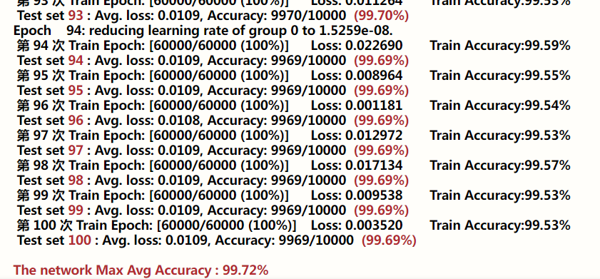
print('\r Test set \033[1;31m{}\033[0m : Avg. loss: {:.4f}, Accuracy: {}/{} \033[1;31m({:.2f}%)\033[0m\n'\
.format(epoch,test_loss, correct,len(test_loader.dataset),100. * acc),end = '')
View the recognition ability of the model
# Let's take a look at the recognition ability of the model. We can see that the performance of the untrained model in the test set is very poor, and the correct recognition rate is only about 10%
test(1)
Training model
### Training!!! And in each epoch Post test ###
###################################################
# According to the number of epochs, formal training was conducted and tested after each epoch training
for epoch in range(1, n_epochs + 1):
    scheduler.step(test_acces[-1])
    train(epoch)
    test(epoch)
#Enter the accuracy of the last saved model, that is, the highest test accuracy
print('\n\033[1;31mThe network Max Avg Accuracy : {:.2f}%\033[0m'.format(100. * max(test_acces)))
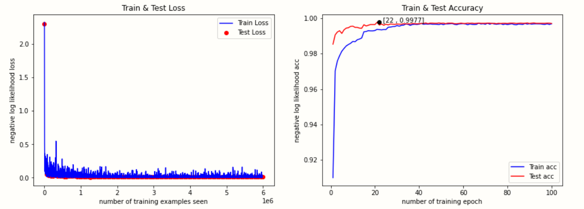
Visual training results
#visualization
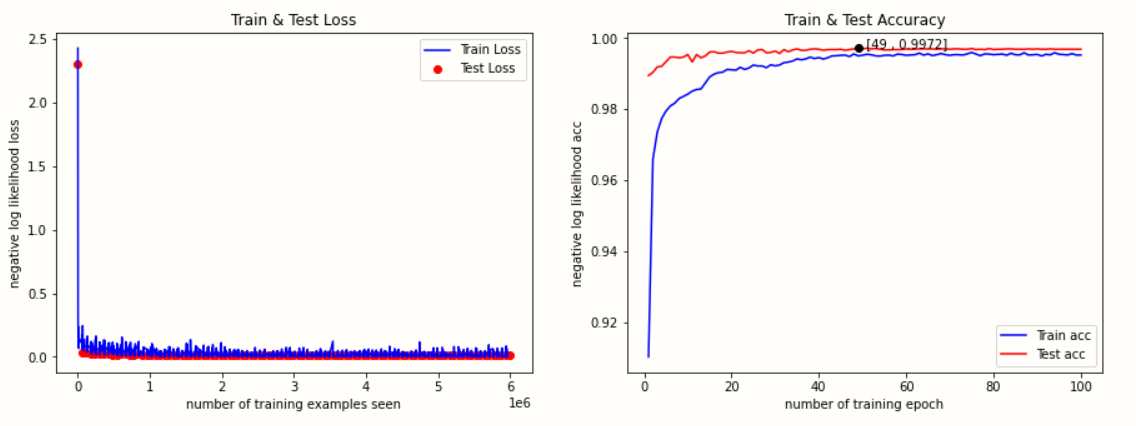
fig = plt.figure(figsize=(15,5))#Enlarge the drawing window 15 times horizontally and 5 times vertically
ax1 = fig.add_subplot(121)
#Training loss
ax1.plot(train_counter, train_losses, color='blue')
#Test loss
plt.scatter(test_counter, test_losses, color='red')
#legend
plt.legend(['Train Loss', 'Test Loss'], loc='upper right')
plt.title('Train & Test Loss')
plt.xlabel('number of training examples seen')
plt.ylabel('negative log likelihood loss')
plt.subplot(122)
#Index of maximum test accuracy
max_test_acces_epoch = test_acces.index(max(test_acces))
#The maximum value is 4 decimal places and rounded
max_test_acces = round(max(test_acces),4)
#Training accuracy
plt.plot([epoch+1 for epoch in range(n_epochs) ], train_acces, color='blue')
#Test accuracy
plt.plot([epoch+1 for epoch in range(n_epochs) ], test_acces[1:], color='red')
plt.plot(max_test_acces_epoch,max_test_acces,'ko') #Maximum point
show_max=' ['+str(max_test_acces_epoch )+' , '+str(max_test_acces)+']'
#Maximum point coordinate display
plt.annotate(show_max,xy=(max_test_acces_epoch,max_test_acces),
xytext=(max_test_acces_epoch,max_test_acces))
plt.legend(['Train acc', 'Test acc'], loc='lower right')
plt.title('Train & Test Accuracy')
#plt.ylim(0.8, 1)
plt.xlabel('number of training epoch')
plt.ylabel('negative log likelihood acc')
plt.show()
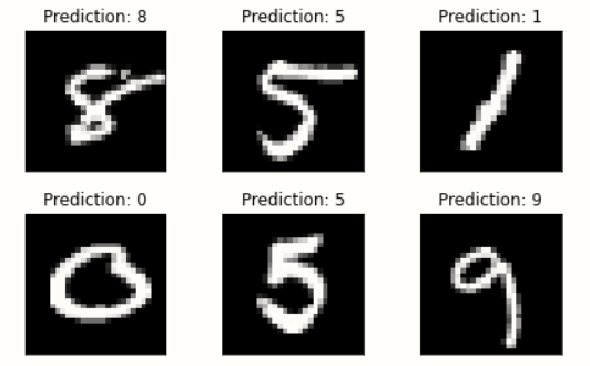
Predict pictures in mnist dataset
#forecast
examples = enumerate(test_loader)
batch_idx, (example_data, example_targets) = next(examples)
with torch.no_grad():
    output = network(example_data.to(device))
    fig = plt.figure()
    for i in range(6):
        plt.subplot(2,3,i+1)
        plt.tight_layout()
        plt.imshow(example_data[i][0], cmap='gray', interpolation='none')
        plt.title("Prediction: {}".format(
        output.data.max(1, keepdim=True)[1][i].item()))
        plt.xticks([])
        plt.yticks([])
    plt.show()
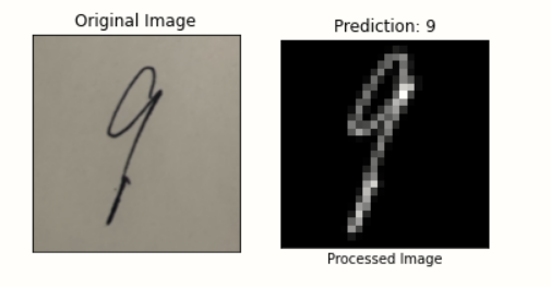
Predicting handwritten digits
Image preprocessing
#Image processing
def imageProcess(img):
    #Processing pictures
    data_transform = torchvision.transforms.Compose(
        [torchvision.transforms.Resize(32),
         torchvision.transforms.CenterCrop(28),
         torchvision.transforms.ToTensor(),
         torchvision.transforms.Normalize((0.1307,), (0.3081,))])

    gray = cv2.cvtColor(img, cv2.COLOR_BGR2GRAY)# Gray processing
    retval, dst = cv2.threshold(gray, 0, 255,cv2.THRESH_BINARY | cv2.THRESH_OTSU)# Binarization
    fanse = cv2.bitwise_not(dst)#Black and white reversal

    #Convert BGR image into RGB image: about CV2 Convert imread to image open
    imgs = Image.fromarray(cv2.cvtColor(fanse, cv2.COLOR_BGR2RGB))
    imgs = imgs.convert('L') #Convert three channel image into single channel gray image
    imgs = data_transform(imgs)#Process image

    return imgs
Loading model
network = CNNModel()
model_path = "./model02.pth"
network.load_state_dict(torch.load(model_path))
network.eval()
Predicted handwritten digits (single sheet)
#Predicting handwritten digits
path = 'E:/jupyter_notebook/test/' #Picture saving path
with torch.no_grad():
    img = cv2.imread(path + '9.jpg')#Forecast picture
    #Call image preprocessing function
    imgs = imageProcess(img)
    if imgs.shape == torch.Size([1,28,28]):
        imgs = torch.unsqueeze(imgs, dim=0) #Add a dimension at the front
    output = network(imgs.to(device))
    plt.tight_layout()
    plt.subplot(121)
    img = Image.fromarray(cv2.cvtColor(img, cv2.COLOR_BGR2RGB))
    plt.imshow(img)
    plt.title("Original Image")
    plt.xticks([])
    plt.yticks([])


    plt.subplot(122)
    plt.imshow(imgs[0][0], cmap='gray', interpolation='none')
    plt.title("Prediction: {}".format(output.data.max(dim = 1, keepdim=True)[1].item()))
    plt.xlabel("Processed Image")
    plt.xticks([])
    plt.yticks([])
    plt.show()
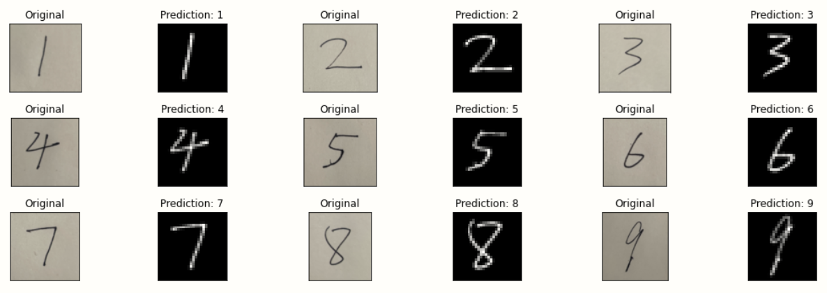
Predicted handwritten digits (multiple)
#Predict multiple handwritten digital pictures
with torch.no_grad():
    fig = plt.figure(figsize=(15,5))

    for i in range(9):
        img = cv2.imread(path + str(i+1) + ".jpg")#Forecast picture
        imgs =  imageProcess(img)
        if imgs.shape == torch.Size([1,28,28]):
            imgs = torch.unsqueeze(imgs, dim=0)
        output = network(imgs)
        ax1 = fig.add_subplot(3,6,2*i+1)
        img = Image.fromarray(cv2.cvtColor(img, cv2.COLOR_BGR2RGB))
        plt.imshow(img)
        plt.title("Original")
        plt.xticks([])
        plt.yticks([])

        plt.subplot(3,6,2*i+2)
        plt.tight_layout()
        plt.imshow(imgs[0][0], cmap='gray', interpolation='none')
        plt.title("Prediction: {}".format(
        output.data.max(dim = 1, keepdim=True)[1].item()))
        plt.xticks([])
        plt.yticks([])
    plt.show()
Adjust parameters and optimize model
Taking the training accuracy as a reference, if there is no increase in one continuous epoch, the learning rate will be reduced
# Instantiate a network
network = CNNModel()
#Loading model
model_path = "./model02.pth"
network.load_state_dict(torch.load(model_path))
network.to(device)

#network.apply(weights_init)

optimizer = optim.RMSprop(network.parameters(),lr=learning_rate,alpha=0.99,momentum = momentum)
scheduler = lr_scheduler.ReduceLROnPlateau(optimizer, mode='max', factor=0.5, patience=1, verbose=True, threshold=1e-06, threshold_mode='rel', cooldown=0, min_lr=0, eps=1e-09)
for epoch in range(101, 201):
    scheduler.step(train_acces[-1])
    train(epoch)
    test(epoch)
print('\n\033[1;31mThe network Max Avg Accuracy : {:.2f}%\033[0m'.format(100. * max(test_acces)))
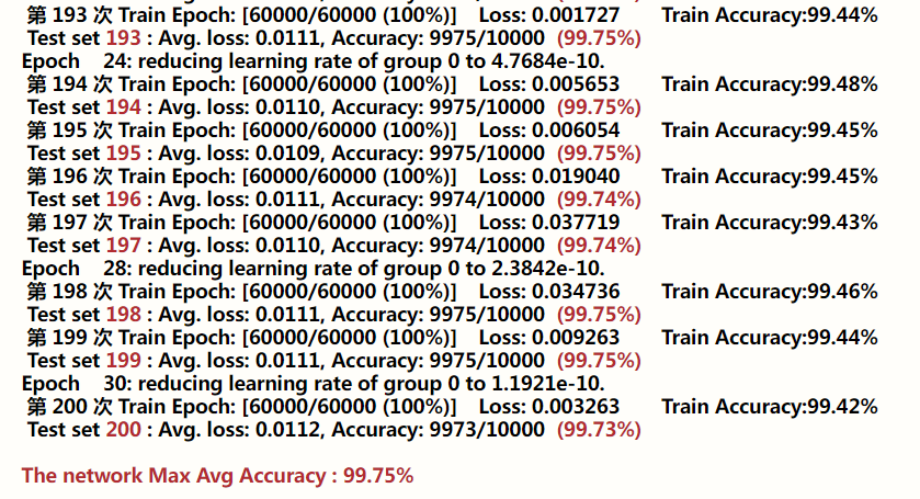
The final accuracy is 99.75%
#Complete prediction code
#Import and storage
import torch
import torchvision
from torch.utils.data import DataLoader
import torch.nn as nn
import torch.nn.functional as F
import torch.optim as optim
import matplotlib.pyplot as plt
from PIL import Image
import matplotlib.image as image
import cv2
import time
import os

#model
class CNNModel(nn.Module):
    def __init__(self):
        super(CNNModel, self).__init__()

        # Convolution layer 1
        self.conv1 = nn.Conv2d(in_channels = 1 , out_channels = 32, kernel_size = 5, stride = 1, padding = 0 )
        self.relu1 = nn.ReLU()
        self.batch1 = nn.BatchNorm2d(32)

        self.conv2 = nn.Conv2d(in_channels =32 , out_channels = 32, kernel_size = 5, stride = 1, padding = 0 )
        self.relu2 = nn.ReLU()
        self.batch2 = nn.BatchNorm2d(32)
        self.maxpool1 = nn.MaxPool2d(kernel_size = 2, stride = 2)
        self.conv1_drop = nn.Dropout(0.25)

        # Convolution layer 2
        self.conv3 = nn.Conv2d(in_channels = 32, out_channels = 64, kernel_size = 3, stride = 1, padding = 0 )
        self.relu3 = nn.ReLU()
        self.batch3 = nn.BatchNorm2d(64)

        self.conv4 = nn.Conv2d(in_channels = 64, out_channels = 64, kernel_size = 3, stride = 1, padding = 0 )
        self.relu4 = nn.ReLU()
        self.batch4 = nn.BatchNorm2d(64)
        self.maxpool2 = nn.MaxPool2d(kernel_size = 2, stride = 2)
        self.conv2_drop = nn.Dropout(0.25)

        # Fully-Connected layer 1

        self.fc1 = nn.Linear(576,256)
        self.fc1_relu = nn.ReLU()
        self.dp1 = nn.Dropout(0.5)

        # Fully-Connected layer 2
        self.fc2 = nn.Linear(256,10)

    def forward(self, x):
        # Forward calculation of conv layer 1, 3 lines of code
        out = self.conv1(x)
        out = self.relu1(out)
        out = self.batch1(out)

        out = self.conv2(out)
        out = self.relu2(out)
        out = self.batch2(out)

        out = self.maxpool1(out)
        out = self.conv1_drop(out)

        # Forward calculation of conv layer 2, 4 lines of code
        out = self.conv3(out)
        out = self.relu3(out)
        out = self.batch3(out)

        out = self.conv4(out)
        out = self.relu4(out)
        out = self.batch4(out)

        out = self.maxpool2(out)
        out = self.conv2_drop(out)

        #Flatten leveling operation
        out = out.view(out.size(0),-1)

        #Forward calculation of FC layer (2 lines of code)
        out = self.fc1(out)
        out = self.fc1_relu(out)
        out = self.dp1(out)

        out = self.fc2(out)

        return F.log_softmax(out,dim = 1)


#Instantiation model
network = CNNModel()

#Loading model
model_path = "./model02.pth"
network.load_state_dict(torch.load(model_path))
network.eval()

#Image processing
def imageProcess(img):
    #Processing pictures
    data_transform = torchvision.transforms.Compose(
        [torchvision.transforms.Resize(32),
         torchvision.transforms.CenterCrop(28),
         torchvision.transforms.ToTensor(),
         torchvision.transforms.Normalize((0.1307,), (0.3081,))])

    gray = cv2.cvtColor(img, cv2.COLOR_BGR2GRAY)# Gray processing
    retval, dst = cv2.threshold(gray, 0, 255,cv2.THRESH_BINARY | cv2.THRESH_OTSU)# Binarization
    fanse = cv2.bitwise_not(dst)#Black and white reversal

    #Convert BGR image into RGB image: about CV2 Convert imread to image open
    imgs = Image.fromarray(cv2.cvtColor(fanse, cv2.COLOR_BGR2RGB))
    imgs = imgs.convert('L') #Convert three channel image into single channel gray image
    imgs = data_transform(imgs)#Process image

    return imgs

#Predict a single handwritten digital picture
path = 'E:/jupyter_notebook/test/'
with torch.no_grad():
    img = cv2.imread(path + '9.jpg')#Forecast picture
    imgs = imageProcess(img)
    if imgs.shape == torch.Size([1,28,28]):
        imgs = torch.unsqueeze(imgs, dim=0) #Add a dimension at the front
    output = network(imgs)
    plt.tight_layout()
    plt.subplot(121)
    img = Image.fromarray(cv2.cvtColor(img, cv2.COLOR_BGR2RGB))
    plt.imshow(img)
    plt.title("Original")
    plt.xticks([])
    plt.yticks([])


    plt.subplot(122)
    plt.imshow(imgs[0][0], cmap='gray', interpolation='none')
    plt.title("Prediction: {}".format(output.data.max(dim = 1, keepdim=True)[1].item()))
    plt.xticks([])
    plt.yticks([])
    plt.show()

"""
#Predict multiple handwritten digital pictures
with torch.no_grad():
    fig = plt.figure(figsize=(15,5))

    for i in range(9):
        img = cv2.imread(path + str(i+1) + ".jpg")#Forecast picture
        imgs =  imageProcess(img)
        if imgs.shape == torch.Size([1,28,28]):
            imgs = torch.unsqueeze(imgs, dim=0)
        output = network(imgs)
        ax1 = fig.add_subplot(3,6,2*i+1)
        img = Image.fromarray(cv2.cvtColor(img, cv2.COLOR_BGR2RGB))
        plt.imshow(img)
        plt.title("Original")
        plt.xticks([])
        plt.yticks([])

        plt.subplot(3,6,2*i+2)
        plt.tight_layout()
        plt.imshow(imgs[0][0], cmap='gray', interpolation='none')
        plt.title("Prediction: {}".format(
        output.data.max(dim = 1, keepdim=True)[1].item()))
        plt.xticks([])
        plt.yticks([])
    plt.show()
"""
Five storey structure
The accuracy of the five layer convolution model is 99.77%. However, due to the deepening of the number of network layers, the training speed becomes much slower.
#model
class CNNModel(nn.Module):
    def __init__(self):
        super(CNNModel, self).__init__()

        # Convolution layer 1
        self.conv1 = nn.Conv2d(in_channels = 1 , out_channels = 64, kernel_size = 5, stride = 1, padding = 2 )
        self.relu1 = nn.ReLU()
        self.batch1 = nn.BatchNorm2d(64)

        self.conv2 = nn.Conv2d(in_channels =64 , out_channels = 64, kernel_size = 5, stride = 1, padding = 2 )
        self.relu2 = nn.ReLU()
        self.batch2 = nn.BatchNorm2d(64)
        self.maxpool1 = nn.MaxPool2d(kernel_size = 2, stride = 2)
        self.drop1 = nn.Dropout(0.25)

        # Convolution layer 2
        self.conv3 = nn.Conv2d(in_channels = 64, out_channels = 64, kernel_size = 3, stride = 1, padding = 1 )
        self.relu3 = nn.ReLU()
        self.batch3 = nn.BatchNorm2d(64)

        self.conv4 = nn.Conv2d(in_channels = 64, out_channels = 64, kernel_size = 3, stride = 1, padding = 1 )
        self.relu4 = nn.ReLU()
        self.batch4 = nn.BatchNorm2d(64)
        self.maxpool2 = nn.MaxPool2d(kernel_size = 2, stride = 2)
        self.drop2 = nn.Dropout(0.25)

        self.conv5 = nn.Conv2d(in_channels = 64, out_channels = 64, kernel_size = 3, stride = 1, padding = 1 )
        self.relu5 = nn.ReLU()
        self.batch5 = nn.BatchNorm2d(64)
        self.drop3 = nn.Dropout(0.25)

        # Fully-Connected layer 1

        self.fc1 = nn.Linear(3136,256)
        self.fc1_relu = nn.ReLU()
        self.batch5 = nn.BatchNorm2d(64)
        self.dp1 = nn.Dropout(0.25)

        # Fully-Connected layer 2
        self.fc2 = nn.Linear(256,10)


    def forward(self, x):
        # Forward calculation of conv layer 1, 3 lines of code
        out = self.conv1(x)
        out = self.relu1(out)
        out = self.batch1(out)

        out = self.conv2(out)
        out = self.relu2(out)
        out = self.batch2(out)

        out = self.maxpool1(out)
        out = self.drop1(out)

        # Forward calculation of conv layer 2, 4 lines of code
        out = self.conv3(out)
        out = self.relu3(out)
        out = self.batch3(out)

        out = self.conv4(out)
        out = self.relu4(out)
        out = self.batch4(out)

        out = self.maxpool2(out)
        out = self.drop2(out)

        out = self.conv5(out)
        out = self.relu5(out)
        out = self.batch5(out)
        out = self.drop3(out)

        #Flatten leveling operation
        out = out.view(out.size(0),-1)

        #Forward calculation of FC layer (2 lines of code)
        out = self.fc1(out)
        out = self.fc1_relu(out)
        out = self.dp1(out)

        out = self.fc2(out)

        return F.log_softmax(out,dim = 1)
Code, model and data set
Link: https://pan.baidu.com/s/1X80lLbKHi-JwiR2L879KeQ
Extraction code: 8igs
reference resources
[1]: Detailed MNIST dataset
[2]: CUDA and cuDNN relationships corresponding to TensorFlow and PyTorch versions
[3]: image transformations for PyTorch learning
[4]:Usage of BatchNorm2d in pytorch
[5]:BN layer of neural network
[6]:Pytorch series – 9 pytorch NN Initialization functions implemented in init: uniform, normal, const, Xavier, He initialization
[7]:Summary of parameter initialization methods in pytorch
[8]:PyTorch learning notes (7): Ten optimizers of PyTorch
[9]:Six learning rate adjustment strategies of PyTorch learning
[10]:Python print() output color setting