This is a plain white book (So Big Readers can move on), and readers can combine videos.
I'm sure you can't see the end of the story.
So see the beginning of the little buddy can point a compliment? *
The little white that is splitting fast
Catalog
Read, display and save pictures
Read, display and save pictures
color image
Each pixel value in the image is divided into three basic color components: B (blue), G (green), R (red). Each basic color component directly determines the intensity of its primary color. The resulting color is called true color. For example, if the image depth is 24 and the color is represented by B:G:R=8:8:8, then R, G, B each occupy 8 bits to represent the intensity of their respective base color components, each of which has a intensity level of 2^8=256. The image can hold 2^24=16M colors (24-bit color). The 24-bit color is called true color, and it reaches the limit of human eye resolution. The number of hairs is 16.77 million colors, which is the 24th power of 2.
Grayscale Image
There is only one sample color image per pixel. Such images are usually displayed as grayscale from the darkest black to the brightest white, with pixels 0-255, the larger the brighter.
#####waitkey() function
cv2.waitkey(delay), the unit of delay is ms milliseconds. When the value of delay is greater than 0, the program waits for user's key trigger within a given delay time. If the user does not press the key, it waits for the next delay time (loop) until user's key triggers and exits the program. If delay is set to 0, then the window interface must be clicked on × To close the program. If the value of delay is set to less than 0 and you wait for the keyboard to press, any key will close the program. The default parameter is less than 0 (printed on my computer is -1). ----------- Copyright Statement: This is an original article by CSDN blogger Yang Jianye, which follows the CC 4.0 BY-SA copyright agreement. Please attach a link to the original source and this statement. Original Link: CV2 in opencv. Detailed waitkey() parameter _ csdn_bajie-CSDN Blog_ cv2.waitkey(0)
Code
'''_read_and_display.py
import cv2
img=cv2.imread('img.jpg',cv2.IMREAD_GRAYSCALE)
print(type(img))
print(img.shape)
'''
cv2.imshow('image',img)
k = cv2.waitKey(0)print(k)
'''
cv2.imwrite('img_gray.jpg',img)
print('yes')
Constants are capitalized: cv2.IMREAD_GRAYSCALE == 0
(At first the imwrite function did not make a mistake but could not generate a picture. Then Mr. Kangkang said that my.py file is in the venv virtual environment, so it's different from the video. Then I clicked "Project" and it suddenly became good.. I don't know what happened.)
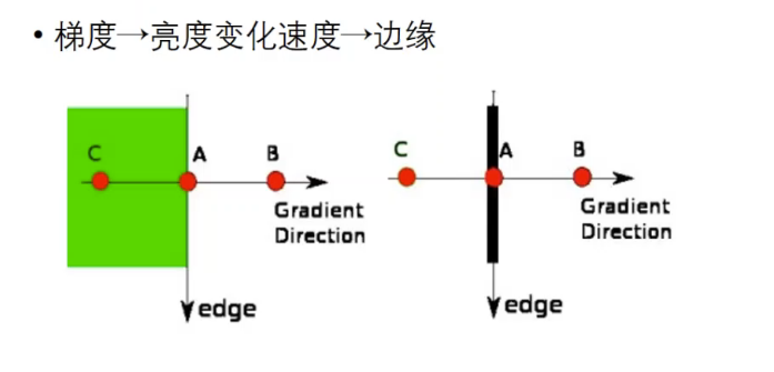
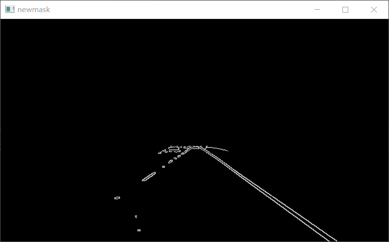
#02Canny Edge Detection
Edge Determination Criteria
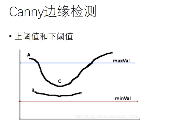
cv2.Canny() function, the first parameter is the input image, the second and third parameters are minVal and maxVal
The weak edge is between the upper and lower thresholds, the strong edge is greater than the upper threshold (we think it must be the edge), and the strong edge connected to the weak edge is considered the true edge:
Consider c as the edge and b as the noise in the figure above.
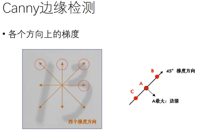
Select four gradient directions (actually eight because there are positive and negative)
Code
'''_edge_detect.py
import cv2
img = cv2.imread('img.jpg',cv2.IMREAD_GRAYSCALE)
edge_img=cv2.Canny(img,70,120)
cv2.imshow('edges',edge_img)
cv2.waitKey(0)
#03.roi_mask
.ROI (region of interest)
Array slices
Boolean operations (and operations)
np.zeros_like(a): Build an array with the same dimension as a and initialize it to 0.
fillPolly function
fillPolly(img,ppt,npt,1,Scalar(255,255,255),lineType)
Function parameters:
1. Polygons will be drawn on img
2. The vertex set of a polygon is ppt (order of points of interest)
3. Draw a polygon with npt vertices
4. The number of polygons to be drawn is 1
5. The color of the polygon is defined as Scarlar(255,255,255), i.e. the RGB value is white
Note: The point boundaries are bracketed
Color principle:
Bitwise AND: Because the white part of the ROI area in the mask picture, 255 (binary 1111111, so sum with this part is still the original number,
But the non-ROI areas are black, that is, 00000000, and when they are in phase 0, they become 0, that is, the uninteresting parts become black
numpy.array function:
A common error includes calling array with multiple numeric parameters instead of providing a list of numeric values as a parameter.
>>> a = array(1,2,3,4) # WRONG >>> a = array([1,2,3,4]) # RIGHT
An array converts a sequence containing sequences into a two-dimensional array, a sequence containing sequences into a three-dimensional array, and so on.
>>> b = array( [ (1.5,2,3), (4,5,6) ] )
>>> b
array([[ 1.5,  2. ,  3. ],
       [ 4. ,  5. ,  6. ]])
Array type can display the specified at creation time
>>> c = array( [ [1,2], [3,4] ], dtype=complex )
>>> c
array([[ 1.+0.j,  2.+0.j],
       [ 3.+0.j,  4.+0.j]])
Another one is very detailed:
Numpy. The array function details Android's nascent blog, CSDN blog np.array function
bitwise_and function
Function prototype: bitwise_and(src1, src2, dst=None, mask=None)
Parameter Description:.src1, src2: For input image or scalar, scalar can be a single value or a quaternion / dst: Optional output variable, defined first if non-None is required, and its size is the same as input variable / mask: image mask, optional parameter, 8-bit single-channel grayscale image, used to specify elements of the output image array to be changed. That is, the output image pixel is only output if the mask corresponding location element is not 0, otherwise all channel components of the location pixel are set to 0
Code
'''roi_mask.py
import cv2
import numpy as np
edge_img =cv2.imread('img.jpg',cv2.IMREAD_GRAYSCALE)
mask = np.zeros_like(edge_img)
mask2 = cv2.fillPoly(mask,np.array([[[0,368],[280,210],[360,210],[640,368]]]),color=255)
masked_edge_img = cv2.bitwise_and(edge_img, mask2)
cv2.imshow('newmask',masked_edge_img)
cv2.waitKey(0)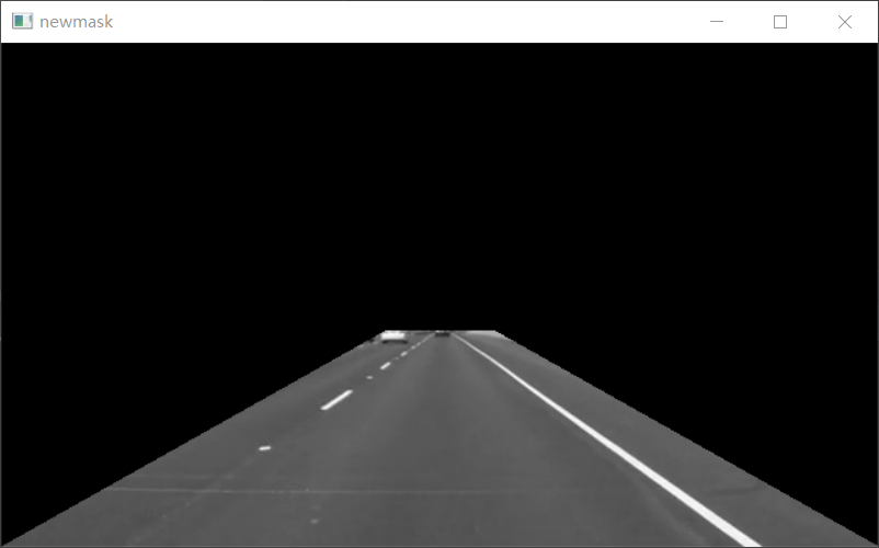
Hoff transformation
Hoff transformation (one: Cartesian coordinates-->Polar coordinates to find the intersection of curves
Binary Image
Binary images (also represented as black and white, B&W, monochrome images) are digital images with only two possible values (0 or 225) per pixel. However, it can also be used to represent any image that has only one sample value per pixel, such as a grayscale image. Binary images can only show edge information.
cv2.line()
For Drawing Lines
cv2.line(img, pt1, pt2, color[, thickness[, lineType[, shift]]]) → img
Impg, Background Diagram. pt1, Line Start Coordinate. pt2, Line End Coordinate. color, color of the current painting. In BGR mode, the pass (255,0,0) represents the blue brush. In a grayscale image, only the brightness value needs to be transferred. Thickness, the thickness and width of the brush. If -1 means drawing a closed image, such as a filled circle. The default value is 1.. lineType, the type of line, such as 8-connected type, anti-aliased line (anti-aliased), is 8-connected style ide by default, cv2.LINE_AA stands for anti-aliasing lines and provides better visual effect when curved.
Note: pt1, pt2 must be tuple, not list
cv2.HoughLinesP()
lines = cv2.HoughLinesP(image, rho, theta, threshold, minLineLength, maxLineGap)
The image is the input image, that is, the source image, which must be a single-channel binary image of 8 units. For other types of images, it is necessary to modify them to this specified format before Hoff transformation can be performed.
< rho is the accuracy of distance r in pixels. Generally, the precision used is 1. (The larger the value, the more lines to consider.)
The TA is an angle θ Accuracy. In general, the precision used is np.pi/180, which means to search for all possible angles.
The threshold is the threshold value. The smaller the value, the more straight lines are determined. The larger the value, the fewer straight lines will be determined.
[When identifying a straight line, determine how many points are located on it. When determining whether a straight line exists, evaluate the number of points that a straight line passes through. If the number of points that a straight line passes through is less than the threshold, these points are considered to be just (accidental) Algorithmically, a straight line is formed, but it does not exist in the source image. Lines are considered to exist if they are greater than the threshold value)
The minLineLength controls the value of "Minimum Length to Accept a Line", with a default value of 0.
The maxLineGap controls the minimum distance between accepted collinear segments, that is, the maximum distance between two points in a line.
If the interval between two points exceeds the value of the parameter maxLineGap, the two points are considered not on the same line. The default value is 0.
Return values: x1,y1,x2,y2.
[ np.array ( [ [x1, y1, x2, y2] ]),
np.array ( [ [x1, y1, x2, y2] ]),
...,
np.array ( [ [x1, y1, x2, y2] ]) ]
Copyright Statement: This is an original article by CSDN blogger Jiangnan Crayon Xiaoxin, which follows the CC 4.0 BY-SA copyright agreement. Please attach a link to the source of the original text and this statement. Original Link: Differences between [OpenCV] HoughLines and HoughLinesP and the display of different effects_ Jiangnan Crayon Xiaoxin-CSDN Blog_ cv2.houghlines
Code
'''
import cv2
import numpy as np
def calculate_slope(line):
    '''    Function: Calculate segments line Slope of
    :param line: np.arry([[x1,y1,x2,y2]])
    :return:
    '''
    x1,y1,x2,y2=line[0]
    return (y1-y2)/(x1-x2)
def reject_abnormal_lines(lines,threshold):
    '''    Exclude line segments with slope outliers
    :param lines: Segment collection,[np.array([[x1, y1, x2, y2]]),...]
    :param threshold: Allow minimum error
    :return:Line segments with consistent slope in error
    '''
    slopes = [calculate_slope(line)for line in lines]
    while len(lines) > 0:
        mean = np.mean(slopes)
        diff = [abs(s - mean)for s in slopes]
        idx = np.argmax(diff)
        if diff[idx] > threshold:
            slopes.pop(idx)
            lines.pop(idx)
            else:
                break
                return lines
            edge_img=cv2.imread('masked_edge.jpg',cv2.IMREAD_GRAYSCALE)
            lines = cv2.HoughLinesP(edge_img,1,np.pi/180,15, minLineLength=40,maxLineGap=20)
            left_lines = [line for line in lines if calculate_slope(line)>0]
            right_lines = [line for line in lines if calculate_slope(line)<0]
    print(len(lines))
    print(len(left_lines))
    print(len(right_lines))
    reject_abnormal_lines(left_lines,0.07)
    reject_abnormal_lines(right_lines,0.07)
    print(len(left_lines))
    print(len(right_lines))
Outlier filtering
show me the code!
'''
import cv2
import numpy as np
def calculate_slope(line):
    '''    Function: Calculate segments line Slope of
    :param line: np.arry([[x1,y1,x2,y2]])
    :return:
    '''
    x1,y1,x2,y2=line[0]
    return (y1-y2)/(x1-x2)
def reject_abnormal_lines(lines,threshold):
    '''    Exclude line segments with slope outliers
    :param lines: Segment collection,[np.array([[x1, y1, x2, y2]]),...]
    :param threshold: Allow minimum error
    :return:Line segments with consistent slope in error
    '''
    slopes = [calculate_slope(line)for line in lines]
    while len(lines) > 0:
        mean = np.mean(slopes)  #Average slope
        diff = [abs(s - mean)for s in slopes]
        idx = np.argmax(diff)   #Slope element subscript for maximum difference
        if diff[idx] > threshold:
            slopes.pop(idx)
            lines.pop(idx)
        else:
            break
    return lines
edge_img=cv2.imread('masked_edge.jpg',cv2.IMREAD_GRAYSCALE)
lines = cv2.HoughLinesP(edge_img,1,np.pi/180,15, minLineLength=40,maxLineGap=20)
#Note that the slope here is the opposite of what we normally do
left_lines = [line for line in lines if calculate_slope(line)<0]
right_lines = [line for line in lines if calculate_slope(line)>0]
print(len(lines))
print(len(left_lines))
print(len(right_lines))
reject_abnormal_lines(left_lines,0.07)
reject_abnormal_lines(right_lines,0.07)
print(len(left_lines))
print(len(right_lines))
Least Squares Fitting
polyfit() and polyval()
Polyvals are evaluation functions
polyfit is a curve fitting function, mainly used for polynomial curve fitting
p = polyfit(x, y, m)
Where x, y are the horizontal and vertical coordinates of the known data point vectors, m is the number of times to fit the polynomial, and the result returns the coefficient of the m-order fitting polynomial, which is stored in the vector p from the highest to the lowest.
y_0 = polyval(p, x_0)
The polynomial can be obtained in x_ The value at 0 is y_0
For example: Input
p = [4 2 1]
x = [5 6 7]
polyval(p, x)
You can get the value of the polynomial p(x)= 4 * x^2+2*x+1 at x=[56 7]
np.ravel()
Reduce the multidimensional array to one dimension.
code snippet
'''
def least_squares_fit(lines):
"""
	take lines Fit a segment in
	:param lines: Segment Collection, [np.array([[x_1, y_1, x_2, y_2]]),np.array([[x_1, y_1, x_2, y_2]]),...,np.array([[x_1, y_1, x_2, y_2]])]
    :return: Two points on a segment,np.array([[xmin, ymin], [xmax, ymax]])
"""
	# 1. Remove all coordinate points
    x_coords = np.ravel([[line[0][0], line[0][2]] for line in lines])
    y_coords = np.ravel([[line[0][1], line[0][3]] for line in lines])
    # 2. Line fitting. Get polynomial coefficients
    poly = np.polyfit(x_coords, y_coords, deg=1)
    # 3. Calculate points on two straight lines based on the polynomial coefficients to uniquely determine the line
    point_min = (np.min(x_coords), np.polyval(poly, np.min(x_coords)))
    point_max = (np.max(x_coords), np.polyval(poly, np.max(x_coords)))
    return np.array([point_min, point_max], dtype=np.int)
print("left lane")
print(least_squares_fit(left_lines))
print("right lane")
print(least_squares_fit(right_lines))
#07 Draw a straight line
plus:(Draw all kinds of straight line problems) See cv2.line()
1. Because the upper left corner is the origin, k>0 goes from top left to bottom right, which is the opposite of what we normally do.
2. About straight line color, cv2.imread() reads in BGR format, not our most common RGB format, i.e. (255,0,0) is blue and not red.
#08 Video Stream Read-Write
Read each frame of the video in a continuous loop
1. Basic Functions
#1.cap = cv2.VideoCapture()
The parameter in VideoCapture() is 0, which means to open the built-in camera of the notebook, and the parameter is to open the video in the path of the video file.
#2.ret,frame = cap.read()
cap.read() Read the video by frame, ret,frame is cap. The two return values of the read() method. Where RET is a Boolean value, it returns True if the reading frame is correct, and False if the file is read to the end. Frame is the image of each frame and is a three-dimensional matrix.
#3.cv2.resize()
Cv2. Resize (src, dsize[, dst[, fx[, fy[, interpolation]]]) -> DST parameter description:
src: image dsize that needs to be resized: target image size dst: scale scale in fx:w direction of target image interpolation-interpolation method. There are five (omitted).
There are three points to note:
1. The shape of dsize is (w,h), while the shape of the image read by opencv is (h,w) 2. When the parameter dsize is not zero, the size of the dst is dsize. Otherwise, it is determined by the size of the src and the scaling ratio FX and fy. It can be seen that dsize and (fx,fy) cannot be both 0.3. Because dsize does not have a default value, it must be specified, that is, we must set dsize=(0,0) when we use FX and y to control size.
#4.cv2.cvtcolor()
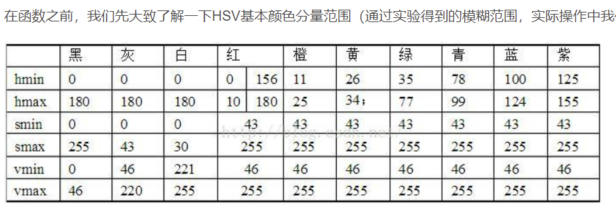
hsv = cv2.cvtColor(rgb_image, cv2.COLOR_BGR2HSV)
#5.cv2.inRange()
mask = cv2.inRange(hsv, lower_red, upper_red)
Parameter description:
hsv: original
lower_red: lower than lower_in the image Value of red, image value becomes 0
upper_red: higher than upper_in the image Value of red, image value becomes 0
2. Slider bar
cv2.createTrackbar()
Function: Bind slider bar and window to define scrollbar value.
cv2.createTrackbar("scale", "display", 0, 100, self.opencv_calibration_node.on_scale)
* Parameter meaning: *
-
First parameter: the name of the slider bar,
-
Second parameter: the name of the window where the slider bar is placed,
-
Third parameter: slider default value,
-
Fourth parameter: the maximum value of the slider bar,
-
The fifth parameter is the callback function, which is called each time you slide.
cv2.getTrackbarPos()
Function: Get the numeric value of the slider bar.
cv2.getTrackbarPos("hue min", "TrackBars")
Parameters:
The first parameter is the name of the slider bar.
Second is the window.
Return value is the value of the slider bar
cv2.setTrackbarPos()
Function: Set the default value of the slider bar.
cv2.setTrackbarPos('Alpha', 'image', 100)
Parameters:
-
The first parameter is the name of the slider bar.
-
The second is the window where s is located.
-
The third parameter is the slider default value.
Attachment: