In this article, we will learn the graph feature learning method based on graph neural network. Graph feature learning requires generating a vector as the representation of the graph according to the node attributes, edges and edge attributes (if any). Based on graph representation, we can predict the graph.
The graph representation network based on graph isomorphism network (GIN) is the most classical graph representation learning network at present. We will take it as an example to learn the graph representation learning method based on graph neural network from three aspects: the implementation of the network, project practice and theoretical analysis.
Implementation of graph signature network
Graph feature learning based on graph isomorphic network mainly includes the following two processes:
-
Firstly, the node representation is calculated;
-
Secondly, Graph Pooling, or Graph Readout, is done for the representation of each node on the graph to obtain Graph Representation.
In this paper, we will adopt a top-down approach to learn the graph feature learning method based on graph isomorphism model (GIN). We first focus on how to get the representation of graph based on node representation calculation, but ignore the method of calculating node representation.
Project practice
Graph representation module based on graph isomorphic network
Firstly, GINNodeEmbedding module is used to embed each node in the graph to get the representation of the node; Then, the node representation is pooled to obtain the representation of the graph; Finally, a layer of linear transformation is used to transform the representation of the graph into the prediction of the graph.
Node embedding - node representation - graph pooling - graph representation - linear transformation
The code implementation is as follows:
import torch
from torch import nn
from torch_geometric.nn import global_add_pool, global_mean_pool, global_max_pool, GlobalAttention, Set2Set
from gin_node import GINNodeEmbedding

class GINGraphRepr(nn.Module):

    def __init__(self, num_tasks=1, num_layers=5, emb_dim=300, residual=False, drop_ratio=0, JK="last", graph_pooling="sum"):
        """GIN Graph Pooling Module
        Args:
            num_tasks (int, optional): number of labels to be predicted. Defaults to 1 (Controls the dimension of graph representation, dimension of graph representation).
            num_layers (int, optional): number of GINConv layers. Defaults to 5.
            emb_dim (int, optional): dimension of node embedding. Defaults to 300.
            residual (bool, optional): adding residual connection or not. Defaults to False.
            drop_ratio (float, optional): dropout rate. Defaults to 0.
            JK (str, optional): The optional values are"last"and"sum". choose"last",Only take the embedding of the last layer of nodes, and select"sum"Sum the embedded nodes of each layer. Defaults to "last".
            graph_pooling (str, optional): pooling method of node embedding. The optional values are"sum","mean","max","attention"and"set2set".  Defaults to "sum".

        Out:
            graph representation
        """
        super(GINGraphPooling, self).__init__()

        self.num_layers = num_layers
        self.drop_ratio = drop_ratio
        self.JK = JK
        self.emb_dim = emb_dim
        self.num_tasks = num_tasks

        if self.num_layers < 2:
            raise ValueError("Number of GNN layers must be greater than 1.")

        self.gnn_node = GINNodeEmbedding(num_layers, emb_dim, JK=JK, drop_ratio=drop_ratio, residual=residual)

        # Pooling function to generate whole-graph embeddings
        if graph_pooling == "sum":
            self.pool = global_add_pool
        elif graph_pooling == "mean":
            self.pool = global_mean_pool
        elif graph_pooling == "max":
            self.pool = global_max_pool
        elif graph_pooling == "attention":
            self.pool = GlobalAttention(gate_nn=nn.Sequential(
                nn.Linear(emb_dim, emb_dim), nn.BatchNorm1d(emb_dim), nn.ReLU(), nn.Linear(emb_dim, 1)))
        elif graph_pooling == "set2set":
            self.pool = Set2Set(emb_dim, processing_steps=2)
        else:
            raise ValueError("Invalid graph pooling type.")

        if graph_pooling == "set2set":
            self.graph_pred_linear = nn.Linear(2*self.emb_dim, self.num_tasks)
        else:
            self.graph_pred_linear = nn.Linear(self.emb_dim, self.num_tasks)

    def forward(self, batched_data):
        h_node = self.gnn_node(batched_data)

        h_graph = self.pool(h_node, batched_data.batch)
        output = self.graph_pred_linear(h_graph)

        if self.training:
            return output
        else:
            # At inference time, relu is applied to output to ensure positivity
            # Because the value range of the prediction target is within (0, 50]
            return torch.clamp(output, min=0, max=50)
Ginnode embedding module based on graph isomorphic network
The node attribute entered into this node embedded module is a category vector.
Steps:
1) Embedded. The input vector is embedded with AtomEncoder to obtain the node representation of layer 0 (we will analyze AtomEncoder later);
2) Compute node characterization. From layer 1 to num_ The layers layer calculates the node representation layer by layer. (the calculation of node representation of each layer takes the node representation h_list[layer], edge_index and edge_attr of the upper layer as inputs).
Note: the more layers of GINConv, the larger the receptive field of the embedded module of this node, and the farthest representation of node i can capture node I is num_ Information of adjacent nodes of layers.
import torch
from mol_encoder import AtomEncoder
from gin_conv import GINConv
import torch.nn.functional as F

# GNN to generate node embedding
class GINNodeEmbedding(torch.nn.Module):
    """
    Output:
        node representations
    """

    def __init__(self, num_layers, emb_dim, drop_ratio=0.5, JK="last", residual=False):
        """GIN Node Embedding Module"""

        super(GINNodeEmbedding, self).__init__()
        self.num_layers = num_layers
        self.drop_ratio = drop_ratio
        self.JK = JK
        # add residual connection or not
        self.residual = residual

        if self.num_layers < 2:
            raise ValueError("Number of GNN layers must be greater than 1.")

        self.atom_encoder = AtomEncoder(emb_dim)

        # List of GNNs
        self.convs = torch.nn.ModuleList()
        self.batch_norms = torch.nn.ModuleList()

        for layer in range(num_layers):
            self.convs.append(GINConv(emb_dim))
            self.batch_norms.append(torch.nn.BatchNorm1d(emb_dim))

    def forward(self, batched_data):
        x, edge_index, edge_attr = batched_data.x, batched_data.edge_index, batched_data.edge_attr

        # computing input node embedding
        h_list = [self.atom_encoder(x)]  # Firstly, the category atomic attribute is transformed into atomic representation
        for layer in range(self.num_layers):
            h = self.convs[layer](h_list[layer], edge_index, edge_attr)
            h = self.batch_norms[layer](h)
            if layer == self.num_layers - 1:
                # remove relu for the last layer
                h = F.dropout(h, self.drop_ratio, training=self.training)
            else:
                h = F.dropout(F.relu(h), self.drop_ratio, training=self.training)

            if self.residual:
                h += h_list[layer]

            h_list.append(h)

        # Different implementations of Jk-concat
        if self.JK == "last":
            node_representation = h_list[-1]
        elif self.JK == "sum":
            node_representation = 0
            for layer in range(self.num_layers + 1):
                node_representation += h_list[layer]

        return node_representation
GINConv -- graph isomorphic convolution
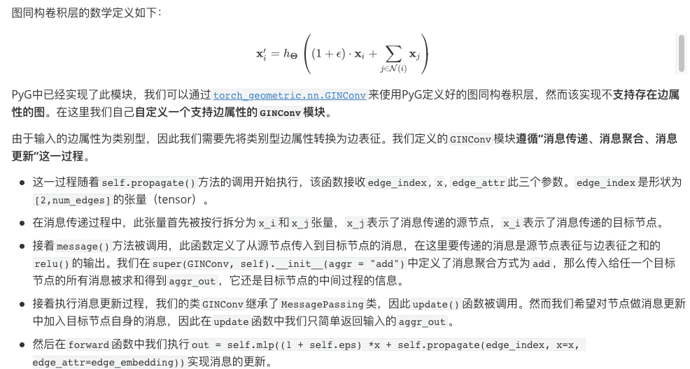
import torch
from torch import nn
from torch_geometric.nn import MessagePassing
import torch.nn.functional as F
from ogb.graphproppred.mol_encoder import BondEncoder


### GIN convolution along the graph structure
class GINConv(MessagePassing):
    def __init__(self, emb_dim):
        '''
            emb_dim (int): node embedding dimensionality
        '''
        super(GINConv, self).__init__(aggr = "add")

        self.mlp = nn.Sequential(nn.Linear(emb_dim, emb_dim), nn.BatchNorm1d(emb_dim), nn.ReLU(), nn.Linear(emb_dim, emb_dim))
        self.eps = nn.Parameter(torch.Tensor([0]))
        self.bond_encoder = BondEncoder(emb_dim = emb_dim)

    def forward(self, x, edge_index, edge_attr):
        edge_embedding = self.bond_encoder(edge_attr) # First, convert the category edge attribute to edge representation
        out = self.mlp((1 + self.eps) *x + self.propagate(edge_index, x=x, edge_attr=edge_embedding))
        return out

    def message(self, x_j, edge_attr):
        #`message() ` X in function_ j + edge_ The attr ` operation performs the fusion of node information and edge information
        return F.relu(x_j + edge_attr)

    def update(self, aggr_out):
        return aggr_out
AtomEncoder and BondEncoder
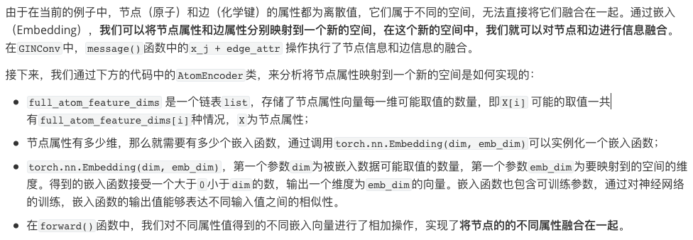
The BondEncoder class is similar to the AtomEncoder class.
import torch
from ogb.utils.features import get_atom_feature_dims, get_bond_feature_dims

full_atom_feature_dims = get_atom_feature_dims()
full_bond_feature_dims = get_bond_feature_dims()

class AtomEncoder(torch.nn.Module):

    def __init__(self, emb_dim):
        super(AtomEncoder, self).__init__()

        self.atom_embedding_list = torch.nn.ModuleList()

        for i, dim in enumerate(full_atom_feature_dims):
            emb = torch.nn.Embedding(dim, emb_dim)
            torch.nn.init.xavier_uniform_(emb.weight.data)
            self.atom_embedding_list.append(emb)

    def forward(self, x):
        x_embedding = 0
        for i in range(x.shape[1]):
            x_embedding += self.atom_embedding_list[i](x[:,i])

        return x_embedding


class BondEncoder(torch.nn.Module):

    def __init__(self, emb_dim):
        super(BondEncoder, self).__init__()

        self.bond_embedding_list = torch.nn.ModuleList()

        for i, dim in enumerate(full_bond_feature_dims):
            emb = torch.nn.Embedding(dim, emb_dim)
            torch.nn.init.xavier_uniform_(emb.weight.data)
            self.bond_embedding_list.append(emb)

    def forward(self, edge_attr):
        bond_embedding = 0
        for i in range(edge_attr.shape[1]):
            bond_embedding += self.bond_embedding_list[i](edge_attr[:,i])

        return bond_embedding


if __name__ == '__main__':
    from loader import GraphClassificationPygDataset
    dataset = GraphClassificationPygDataset(name = 'tox21')
    atom_enc = AtomEncoder(100)
    bond_enc = BondEncoder(100)

    print(atom_enc(dataset[0].x))
    print(bond_enc(dataset[0].edge_attr))
theoretical analysis
Graph isomorphism test
Two graphs are isomorphic, which means that two graphs have the same topology, that is, we can convert from one graph to another by re labeling nodes. The isomorphism testing algorithm of weisfeiler Lehman graphs, WL Test for short, is an algorithm used to test whether two graphs are isomorphic.
Note: WL test cannot guarantee that it is valid for all graphs, especially for graphs with high symmetry, such as chain graph, complete graph, ring graph and star graph.
Weisfeiler Lehman graph kernels method proposes to use WL subtree kernel to measure the similarity between graphs. This method uses the node label count in different iterations of WL Test as the representation vector of the graph, which has the same discrimination ability as WL Test. Intuitively speaking, in the second iteration of WL Test, the label of a node represents the subtree structure with height k with the node as the root.
Figure similarity assessment
This method comes from Weisfeiler-Lehman Graph Kernels.
One limitation of WL Test algorithm is that it can only judge the similarity of two graphs and cannot measure the similarity between graphs. To measure the similarity between the two graphs, we use the WL Subtree Kernel method. The idea of this method is to use WL Test algorithm to obtain multi-layer labels of nodes, and then we can count the times of various labels in the graph and store them in a vector, which can be used as the representation of the graph. The inner product of the characterization vector of two graphs can be used as the similarity estimation of the two graphs. The larger the inner product, the higher the similarity.
Construction of graph isomorphic network model
The graph neural network that can judge graph isomorphism needs to meet the following requirements. Only when the labels of two nodes are the same and their adjacent nodes are the same, the graph neural network maps the two nodes to the same representation, that is, the mapping is injective.
Repeatable sets refer to the sets in which elements can be repeated, and the elements have no sequential relationship in the set. All adjacent nodes of a node are a repeatable set. A node can have duplicate adjacent nodes, and the adjacent nodes have no sequential relationship.
Therefore, the method of generating node representation in GIN model follows the process of updating node label by WL Test algorithm.
After generating the representation of nodes, it is still necessary to perform graph pooling (or graph readout) to obtain graph features. The simplest graph readout operation is summation. Since the node representation of each layer may be important, in a graph isomorphic network, the node representations of different layers are spliced after summation. Its mathematical definition is as follows,

The reason for using splicing rather than adding is that the representation of nodes in different layers belongs to different feature spaces. Without strict proof, the representation of the graph obtained in this way is equivalent to the representation of the graph obtained by WL Subtree Kernel.
summary
In this article, we learned the graph representation network based on graph isomorphic network (GIN). In order to obtain the graph features, we first need to characterize the nodes, and then read the graph.
The calculation of node representation in GIN follows the updating method of node label in WL Test algorithm, so its upper bound is WL Test algorithm.
In graph readout, we sum all node representations (weighted, if Attention is used), which will cause the loss of node distribution information.
task
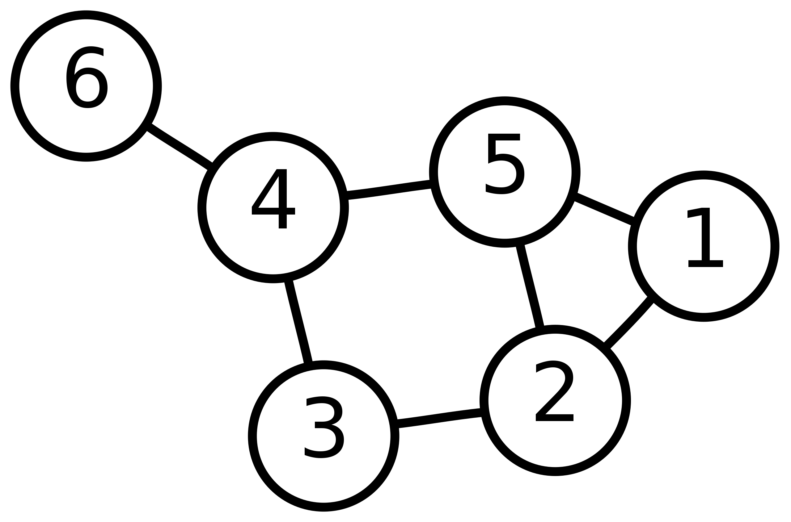
Please draw the WL subtree from layer 1 to layer 3 of nodes 6, 3 and 5 in the picture below.
The WL subtree with height 3 with nodes 6, 3 and 5 as root nodes is shown in the following figure.
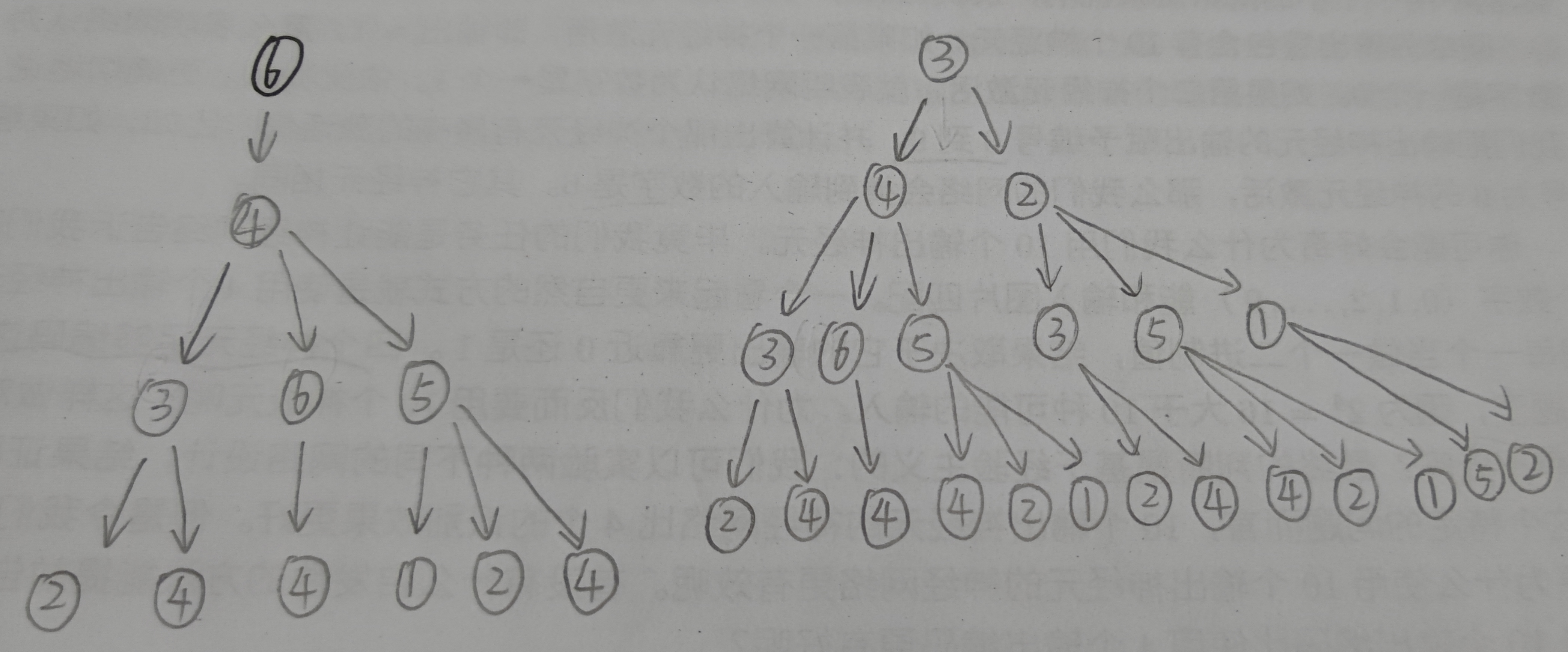
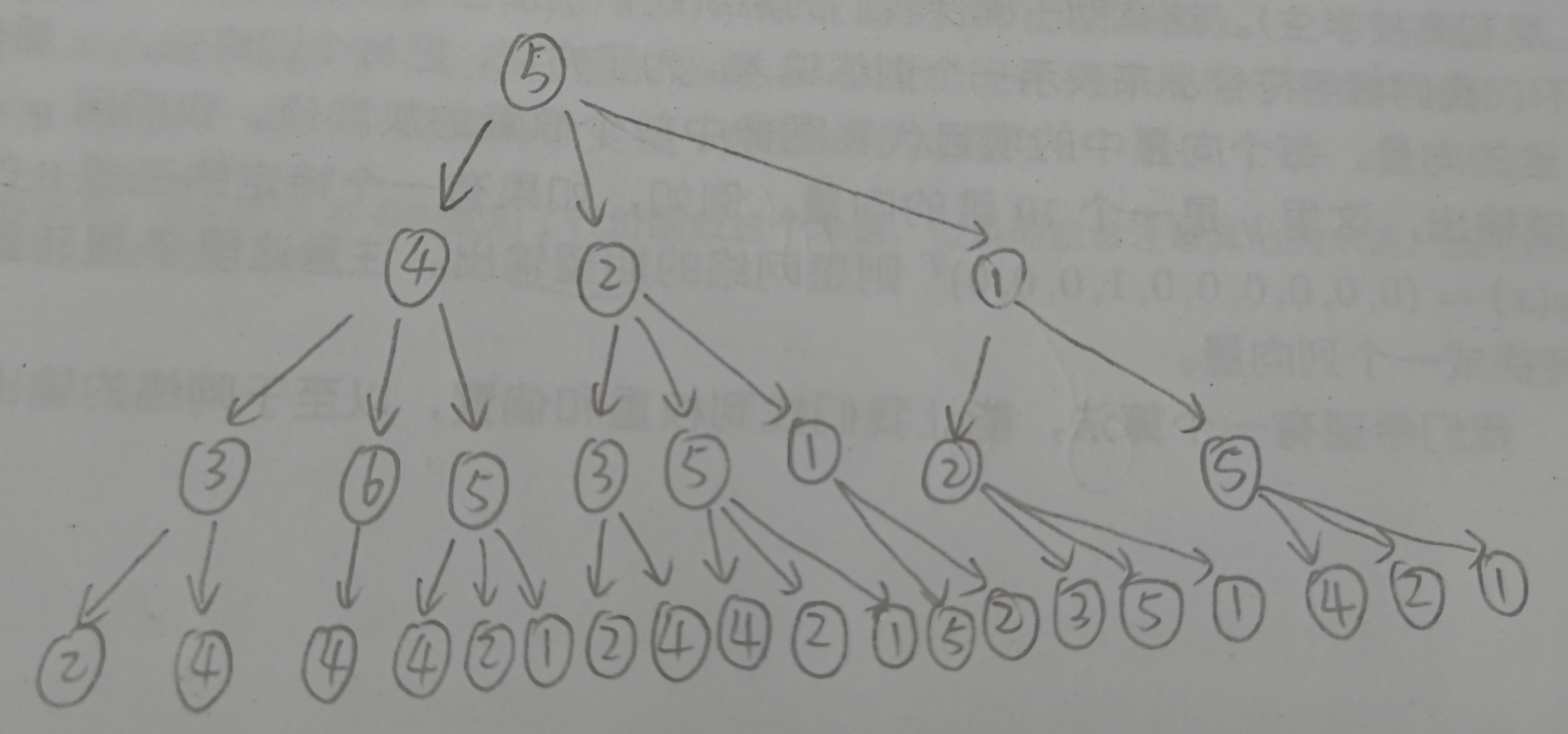
(the picture is a little scrawly, focusing on the content)
reference material
-
Paper on GlobalAttention: "Gated Graph Sequence Neural Networks"
-
Paper on Set2Set: "Order Matters: Sequence to sequence for sets"
-
Methods for pooling all graphs integrated in PyG: Global Pooling Layers
-
Weisfeiler-Lehman Test: Brendan L Douglas. The weisfeiler-lehman method and graph isomorphism testing. arXiv preprint arXiv:1101.5211, 2011.
-
https://github.com/datawhalechina/team-learning-nlp/tree/master/GNN/Markdown edition