1, Introduction

1 Retinex
1.1 theory
Retinex theory began with a series of contributions made by land and McCann in the 1960s. Its basic idea is that the color and brightness of a point perceived by human beings are not only determined by the absolute light entering the human eye, but also related to the color and brightness around it. Retinex is a combination of retina and cortex Land designed the word to show that he did not know whether the characteristics of the visual system depended on either of these two physiological structures or were related to both.
Land's Retinex model is based on the following:

(1) The real world is colorless. The color we perceive is the result of the interaction between light and matter. The water we see is colorless, but the water film soap film is colorful, which is the result of light interference on the surface of the film;
(2) Each color region is composed of red, green and blue primary colors of a given wavelength;
(3) The three primary colors determine the color of each unit area. The ability of the object to reflect X-rays is determined by the absolute intensity of the medium wavelength (red) and the short wavelength (green) rather than the basic intensity of the light; The color of the object is not affected by the non-uniformity of illumination and has consistency, that is, the Retinex theory is based on the consistency of color perception (color constancy). As shown in the figure below, the image S of the object seen by the observer is obtained by the reflection of the object surface on the incident light L, and the reflectivity R is determined by the object itself and is not changed by the incident light L.

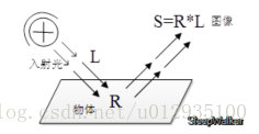
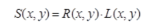
The basic assumption of Retinex theory is that the original image S is the product of illumination image L and reflectivity image R, which can be expressed in the form of the following formula:

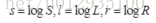
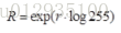
The purpose of Retinex based image enhancement is to estimate the illumination L from the original image S, so as to decompose R and eliminate the influence of uneven illumination, so as to improve the visual effect of the image, just like the human visual system. In processing, the image is usually transferred to the logarithmic domain, i.e

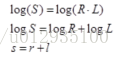
Thus, the product relationship is converted to the relationship of sum:

The core of Retinex method is to estimate the illuminance L, estimate the L component from the image S, and remove the L component to obtain the original reflection component R, that is:

The function f(x) realizes the estimation of the contrast degree L (it can be understood that many actually estimate the r component directly).

2. Understanding of Retinex theory
If you look at the paper, then in the following pages, you will certainly introduce two classic Retinex algorithms: path based Retinex and center / surround based Retinex. Before introducing the two classical Retinex algorithms, I will first talk about my personal understanding, so that friends who come into contact with the theory for the first time can understand it more quickly. Of course, if there is any problem with my understanding, please help me point it out.
As far as I understand, Retinex theory is similar to noise reduction. The key of this theory is to reasonably assume the composition of the image. If the image seen by the observer is regarded as an image with multiplicative noise, the component of incident light is a multiplicative, relatively uniform and slow transformation noise. What Retinex algorithm does is to reasonably estimate the noise at each position in the image and remove it.
In extreme cases, we can think that the components in the whole image are uniform, so the simplest way to estimate the illuminance L is to calculate the mean value of the whole image after transforming the image to the logarithmic domain. Therefore, I designed the following algorithm to verify my conjecture. The process is as follows:
(1) Transform image to log domain

(2) Normalized removal of additive components

(3) Find the exponent of the result obtained in step 3 and inverse transform it to the real number field

2 dark channel
2.1 he Kaiming's dark channel prior defogging algorithm is a well-known algorithm in the field of CV defogging. The paper on this algorithm "Single Image Haze Removal Using Dark Channel Prior" won the best paper of CVPR in 2009. The author counted a large number of fog free images and found a rule: among the three RGB color channels of each image, the gray value of one channel is very low and almost tends to 0. Based on the prior knowledge that can almost be regarded as a theorem, the author proposes a dark channel a priori defogging algorithm.
The mathematical expression of the dark channel is:


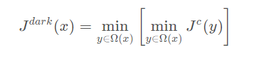
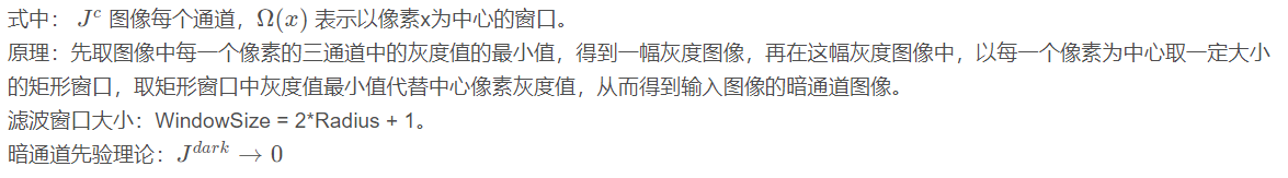
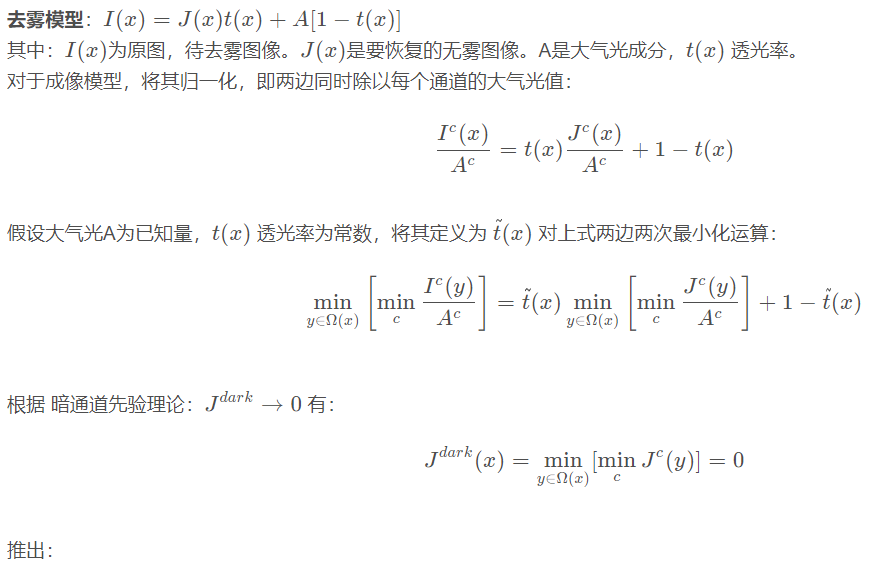
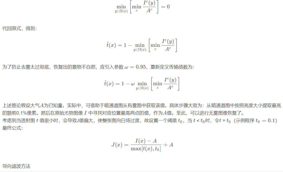
2.1 fog removal principle of dark channel

2, Source code

clc
clear all;
I=imread('C:\Users\lenovo\Desktop\Image defogging algorithm code\Bi design code\fog.jpg');
tic

R=I(:,:,1);
G=I(:,:,2);
B=I(:,:,3);
M=histeq(R);
N=histeq(G);
L=histeq(B);
In=cat(3,M,N,L);

imshow(In);
figure
imshowpair(I, In, 'montage');
t=toc;



[C,L]=size(I); %Find the specification of the image
Img_size=C*L; %Total number of image pixels
G=256; %Gray level of image
H_x=0;
nk=zeros(G,1);%Generate a G All zero matrix of row 1 column
for i=1:C
for j=1:L
Img_level=I(i,j)+1; %Get the gray level of the image
nk(Img_level)=nk(Img_level)+1; %Count the number of points of each gray level pixel
end
end
clear all;
clc;
tic
%1, Image preprocessing, read in the color image and grayscale it
PS=imread('C:\Users\lenovo\Desktop\Image defogging algorithm code\Bi design code\fog.jpg');                %Read in BMP Color image file
imshow(PS)                                  %Show
title('Input image')
%imwrite(rgb2gray(PS),'PicSampleGray.bmp'); %Grayscale and save color pictures
R=PS(:,:,1);                          %The grayed data is stored in the array

%2, Draw histogram
[m,n]=size(R);                             %Measure image size parameters
GP=zeros(1,256);                            %Pre create a vector to store the occurrence probability of gray scale
for k=0:255
     GP(k+1)=length(find(R==k))/(m*n);      %Calculate the probability of each gray level and store it in GP Corresponding position in
end
figure,
bar(0:255,GP,'g')                    %Draw histogram
title('Histogram of fog image')
xlabel('Gray value')
ylabel('Probability of occurrence')
%3, Histogram equalization
S1=zeros(1,256);
for i=1:256
     for j=1:i
          S1(i)=GP(j)+S1(i);                 %calculation Sk
     end
end
S2=round((S1*256)+0.5);                          %take Sk Grayscale assigned to a similar level
for i=1:256
     GPeq(i)=sum(GP(find(S2==i)));           %Calculate the probability of each existing gray level
end
figure,bar(0:255,GPeq,'b')                  %Display the histogram after equalization
title('Histogram after equalization')
xlabel('Gray value')
ylabel('Probability of occurrence')
%4, Image equalization
PA=R;
for i=0:255
     PA(find(R==i))=S2(i+1);                %Assign the normalized gray value of each pixel to this pixel
end




G=PS(:,:,2);                          %The grayed data is stored in the array

%2, Draw histogram
[m,n]=size(R);                             %Measure image size parameters
GPG=zeros(1,256);                            %Pre create a vector to store the occurrence probability of gray scale
for k=0:255
     GPG(k+1)=length(find(G==k))/(m*n);      %Calculate the probability of each gray level and store it in GP Corresponding position in
end

%3, Histogram equalization
SG=zeros(1,256);
for i=1:256
     for j=1:i
          SG(i)=GPG(j)+SG(i);                 %calculation Sk
     end
end
S2G=round((SG*256)+0.5);                          %take Sk Grayscale assigned to a similar level
for i=1:256
     GPeqG(i)=sum(GPG(find(S2G==i)));           %Calculate the probability of each existing gray level
end

%4, Image equalization
PAG=G;
for i=0:255
     PAG(find(G==i))=S2G(i+1);                %Assign the normalized gray value of each pixel to this pixel
end
%figure,imshow(PAG)                           %Display the equalized image
%title('Image after equalization')


B=PS(:,:,3);                          %The grayed data is stored in the array

%2, Draw histogram
[m,n]=size(B);                             %Measure image size parameters
GPB=zeros(1,256);                            %Pre create a vector to store the occurrence probability of gray scale
for k=0:255
     GPB(k+1)=length(find(B==k))/(m*n);      %Calculate the probability of each gray level and store it in GP Corresponding position in
end

%3, Histogram equalization
S1B=zeros(1,256);
for i=1:256
     for j=1:i
          S1B(i)=GPB(j)+S1B(i);                 %calculation Sk
     end
end
S2B=round((S1B*256)+0.5);                          %take Sk Grayscale assigned to a similar level
for i=1:256
     GPeqB(i)=sum(GPB(find(S2B==i)));           %Calculate the probability of each existing gray level
end
clear all;
tic
I = imread('C:\Users\lenovo\Desktop\Image defogging algorithm code\Bi design code\fog.jpg');
R = I(:, :, 1);
 %imhist(R);
% figure;
[N1, M1] = size(R);
R0 = double(R);
Rlog = log(R0+1);
Rfft2 = fft2(R0);
 
sigma = 200;
F = fspecial('gaussian', [N1,M1], sigma); 
Efft = fft2(double(F));
 
DR0 = Rfft2.* Efft;
DR = ifft2(DR0);
 
DRlog = log(DR +1);
Rr = Rlog - DRlog;
EXPRr = exp(Rr);
%imhist(EXPRr);
%figure;
MIN = min(min(EXPRr));
MAX = max(max(EXPRr));
EXPRr = (EXPRr - MIN)/(MAX - MIN)*255;
EXPRr=uint8(EXPRr);
imhist(EXPRr);
figure;
EXPRr = adapthisteq(EXPRr);
% imhist(EXPRr);
%figure;
G = I(:, :, 2);
 
G0 = double(G);
Glog = log(G0+1);
Gfft2 = fft2(G0);
  
DG0 = Gfft2.* Efft;
DG = ifft2(DG0);
 
DGlog = log(DG +1);
Gg = Glog - DGlog;
EXPGg = exp(Gg);
MIN = min(min(EXPGg));
MAX = max(max(EXPGg));
EXPGg = (EXPGg - MIN)/(MAX - MIN)*255;
EXPGg=uint8(EXPGg);
%imhist(EXPGg);
%figure;
EXPGg = adapthisteq(EXPGg);

3, Operation results

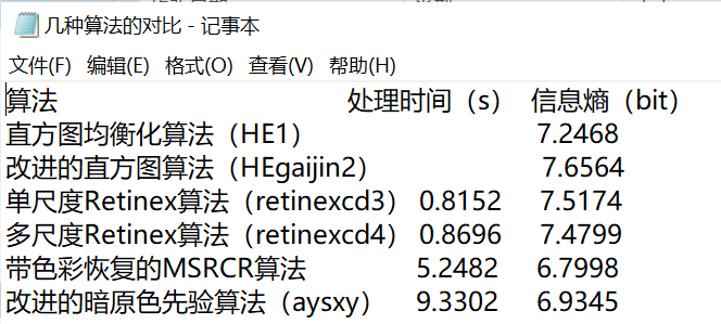
Due to the large number of running results of various algorithms, summary and comparison are provided here:

4, Remarks

Complete code or write on behalf of QQ 912100926