This article is shared from Huawei cloud community< [Python from zero to one] 43 Image point operation and image graying in image enhancement and operation >, by eastmount.
I Concept of image point operation
Image Point Operation refers to that for an input image, an output image will be generated, and the gray value of each pixel of the output image is determined by the input pixel. Point Operation is actually a gray-scale to gray-scale mapping process, which can enhance or weaken the gray-scale of the image through mapping transformation. It can also calculate the gray histogram, linear transformation, nonlinear transformation and image skeleton extraction of the image. It has no operational relationship with adjacent pixels. It is a simple and effective image processing method [1].
The gray-scale transformation of the image can selectively highlight the features of interest or suppress the unwanted features in the image, so as to improve the quality of the image, highlight the details of the image and improve the contrast of the image. It can also effectively change the histogram distribution of the image and make the pixel value distribution of the image more uniform [2-3]. It has many applications in practice:
- photometric calibration
- Contrast enhancement
- Contrast extension
- Display calibration
- Contour determination
If the input image is A(x,y) and the output image is B(x,y), the point operation can be expressed as:
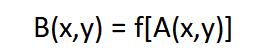
There are differences between image point operation and geometric operation, which will not change the spatial position relationship between pixels in the image. At the same time, it is also different from local (domain) operation. Input pixels and output pixels correspond to each other one by one.
II Image grayscale processing
Image graying is the process of converting a color image into a grayed image. Color image usually includes three components: R, G and B, which display various colors such as red, green and blue respectively. Graying is the process of making the three components of color image equal. Each pixel in the gray-scale image has only one sample color. Its gray-scale is the multi-level color depth between black and white. The pixels with large gray-scale value are brighter, on the contrary, they are darker. The maximum pixel value is 255 (indicating white) and the minimum pixel value is 0 (indicating black).
Assuming that the color of a point is composed of RGB(R,G,B), the common gray processing algorithms are shown in table 11-1:
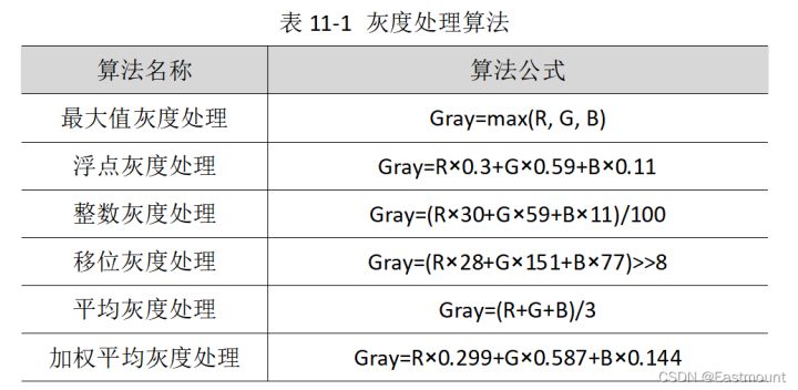
In table 11-1, Gray represents the color after Gray processing, and then the original RGB(R,G,B) color is evenly replaced with the new color RGB(Gray,Gray,Gray), so as to convert the color picture into Gray image. A common method is to sum the three RGB components and then take the average value, but a more accurate method is to set different weights and divide the RGB components into Gray levels according to different proportions. For example, the sensitivity of human eyes to blue is the lowest, and the most sensitive is green. Therefore, a more reasonable Gray image can be obtained by weighted average of RGB according to the proportion of 0.299, 0.587 and 0.144, as shown in formula 11-2 [4-6].

In daily life, most of the color images we see are RGB, but in the process of image processing, we often need to use gray image, binary image, HSV, HSI and other colors. OpenCV provides cvtColor() function to realize these functions. Its function prototype is as follows:
- dst = cv2.cvtColor(src, code[, dst[, dstCn]])
– src refers to the input image and the original image requiring color space transformation
– dst represents the output image, and its size and depth are consistent with src
– code indicates the code or identification of the conversion
– dstCn indicates the number of target image channels. When its value is 0, it is determined by src and code
This function is used to convert an image from one color space to another, where RGB refers to Red, Green and Blue, and an image is composed of these three channels; Gray indicates that there is only one channel of gray Value; HSV contains Hue, Saturation and Value channels.
In OpenCV, common color space conversion identifiers include CVs_ BGR2BGRA,CV_RGB2GRAY,CV_GRAY2RGB,CV_BGR2HSV,CV_BGR2XYZ,CV_BGR2HLS et al. The following is the code that calls the cvtColor() function to grayscale the image.
# -*- coding: utf-8 -*-
# By: Eastmount
import cv2
import numpy as np
#Read original picture
src = cv2.imread('luo.png')
#Image grayscale processing
grayImage = cv2.cvtColor(src,cv2.COLOR_BGR2GRAY)
#Display image
cv2.imshow("src", src)
cv2.imshow("result", grayImage)
#Wait for display
cv2.waitKey(0)
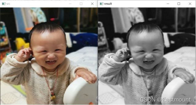
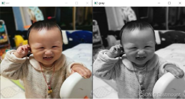
cv2.destroyAllWindows()The output result is shown in Figure 11-1. On the left is the original color "small Luo Luo", and on the right is the grayscale image after grayscale processing of the color image. Among them, the grayscale image sets the three color variables of a pixel to be equal (R=G=B). At this time, this value is called the grayscale value.
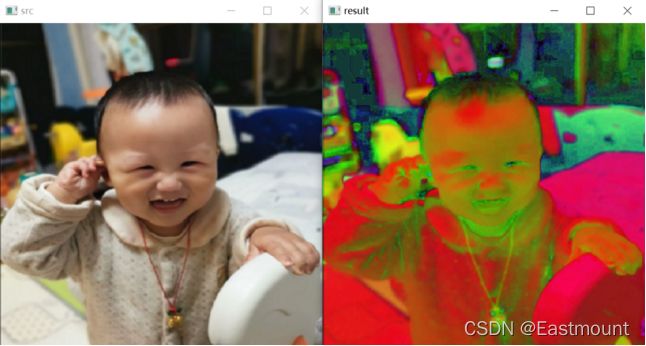
Similarly, the following core code can be called to convert the color image into HSV color space, and the output result is shown in Figure 11-2.
- grayImage = cv2.cvtColor(src, cv2.COLOR_BGR2HSV)
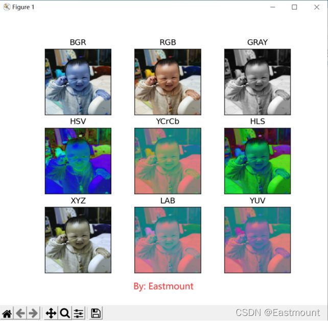
The following code compares nine common color spaces, including BGR, RGB, GRAY, HSV, YCrCb, HLS, XYZ, LAB and YUV, and circulates the processed images.
# -*- coding: utf-8 -*-
# By: Eastmount
import cv2
import numpy as np
import matplotlib.pyplot as plt

#Read original image
img_BGR = cv2.imread('luo.png')

img_RGB = cv2.cvtColor(img_BGR, cv2.COLOR_BGR2RGB)     #Convert BGR to RGB
img_GRAY = cv2.cvtColor(img_BGR, cv2.COLOR_BGR2GRAY)   #Grayscale processing
img_HSV = cv2.cvtColor(img_BGR, cv2.COLOR_BGR2HSV)     #BGR to HSV
img_YCrCb = cv2.cvtColor(img_BGR, cv2.COLOR_BGR2YCrCb) #BGR to YCrCb
img_HLS = cv2.cvtColor(img_BGR, cv2.COLOR_BGR2HLS)     #BGR to HLS
img_XYZ = cv2.cvtColor(img_BGR, cv2.COLOR_BGR2XYZ)     #BGR to XYZ
img_LAB = cv2.cvtColor(img_BGR, cv2.COLOR_BGR2LAB)     #BGR to LAB
img_YUV = cv2.cvtColor(img_BGR, cv2.COLOR_BGR2YUV)     #BGR to YUV

#Call matplotlib to display the processing results
titles = ['BGR', 'RGB', 'GRAY', 'HSV', 'YCrCb', 'HLS', 'XYZ', 'LAB', 'YUV']
images = [img_BGR, img_RGB, img_GRAY, img_HSV, img_YCrCb,
          img_HLS, img_XYZ, img_LAB, img_YUV]
for i in range(9):
   plt.subplot(3, 3, i+1), plt.imshow(images[i], 'gray')
   plt.title(titles[i])
   plt.xticks([]),plt.yticks([])
plt.show()
The operation results are shown in Figure 11-3:
III Image grayscale processing based on pixel operation
Previously, we talked about the processing of image graying by calling cvtColor() function in OpenCV. Next, we explained the image graying processing methods based on pixel operation, mainly the maximum grayscale processing, average grayscale processing and weighted average grayscale processing methods.
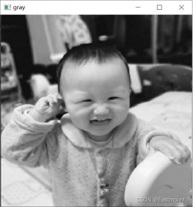
1. Maximum gray processing method
The gray value of this method is equal to the maximum value of the three components of color image R, G and B. the formula is as follows:

The grayscale image after grayscale processing has high brightness. The implementation code is as follows.
# -*- coding: utf-8 -*-
# By: Eastmount
import cv2
import numpy as np
import matplotlib.pyplot as plt

#Read original image
img = cv2.imread('luo.png')

#Get image height and width
height = img.shape[0]
width = img.shape[1]

#Create an image
grayimg = np.zeros((height, width, 3), np.uint8)

#Image maximum gray processing
for i in range(height):
    for j in range(width):
        #Get image R G B Max
        gray = max(img[i,j][0], img[i,j][1], img[i,j][2])
        #Gray image pixel assignment gray=max(R,G,B)
        grayimg[i,j] = np.uint8(gray)

#Display image
cv2.imshow("src", img)
cv2.imshow("gray", grayimg)
#Wait for display
cv2.waitKey(0)
cv2.destroyAllWindows()
The output result is shown in Figure 11-4, and the gray level of the processing effect is too bright.
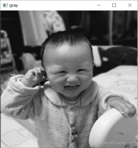
2. Average gray processing method
The gray value of this method is equal to the sum average of the gray values of the three components of color image R, G and B. the calculation formula is shown in formula (11-4):
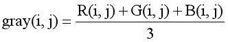
The implementation code of the average gray processing method is as follows.
# -*- coding: utf-8 -*-
# By: Eastmount
import cv2
import numpy as np
import matplotlib.pyplot as plt

#Read original image
img = cv2.imread('luo.png')

#Get image height and width
height = img.shape[0]
width = img.shape[1]

#Create an image
grayimg = np.zeros((height, width, 3), np.uint8)

#Gray average image processing method
for i in range(height):
    for j in range(width):
        #The gray value is the average of three RGB components
        gray = (int(img[i,j][0]) + int(img[i,j][1]) + int(img[i,j][2]))  /  3
        grayimg[i,j] = np.uint8(gray)

#Display image
cv2.imshow("src", img)
cv2.imshow("gray", grayimg)

#Wait for display
cv2.waitKey(0)
cv2.destroyAllWindows()
The output results are shown in Figure 11-5:
3. Weighted average gray processing method
According to the color importance, the three components are weighted and averaged with different weights. Because the human eye is most sensitive to green and least sensitive to blue, a reasonable gray image can be obtained by weighted averaging the RGB three components according to the following formula.

The implementation code of weighted average gray processing method is as follows:
# -*- coding: utf-8 -*-
# By: Eastmount
import cv2
import numpy as np
import matplotlib.pyplot as plt

#Read original image
img = cv2.imread('luo.png')

#Get image height and width
height = img.shape[0]
width = img.shape[1]

#Create an image
grayimg = np.zeros((height, width, 3), np.uint8)

#Gray average image processing method
for i in range(height):
    for j in range(width):
        #Gray weighted average method
        gray = 0.30 * img[i,j][0] + 0.59 * img[i,j][1] + 0.11 * img[i,j][2]
        grayimg[i,j] = np.uint8(gray)

#Display image
cv2.imshow("src", img)
cv2.imshow("gray", grayimg)

#Wait for display
cv2.waitKey(0)
cv2.destroyAllWindows()
The output results are shown in Figure 11-6:
IV summary
This paper mainly explains the grayscale processing of image point operation, introduces the commonly used grayscale processing methods in detail, and shares the mutual conversion of image color space and the implementation of three grayscale conversion algorithms. Through gray-scale processing, we can effectively convert color images into gray-scale images, provide support for subsequent edge extraction and other processing, and may also realize the simplest color image to black-and-white effect of image processing software. I hope it will be helpful to you.
Click follow to learn about Huawei's new cloud technology for the first time~