# Download skimage
pip install scikit-image -i http://pypi.douban.com/simple/ --trusted-host pypi.douban.com
1, Installation of ipython
#Install ipython
pip install ipython
# Enter the ipython command line
ipython
2, Installation and configuration of Jupiter notebook
Jupiter notebook is a note taking tool for writing python code and saving running results. It is very convenient.
1. Installation and startup of jupyter
# Installing jupyter
pip install jupyter
# Start Jupiter notebook
jupyter notebook
2. Common configuration of Jupiter notebook
The default file saving location of jupyter notebook is generally on Disk C, and we generally don't want to save. ipynb note files on Disk C, so we need to customize the file saving location.
- Enter the command window and enter Jupiter notebook -- generate config to generate a configuration file. The generated configuration file is generally in Jupiter under the C: \ users \ liulushing \. Jupiter folder_ notebook_ Config.py.
# Generate configuration file for Jupiter notebook
jupyter notebook --generate-config
- Find the configuration file, open it with an editor, and find c.NotebookApp.notebook_dir and open the comment and replace it with the path to save to.
c.NotebookApp.notebook_dir = 'D:\jupyter-notebook'
- Just restart Jupiter notebook.
# Start Jupiter notebook
jupyter notebook
3, Use of matplotlib
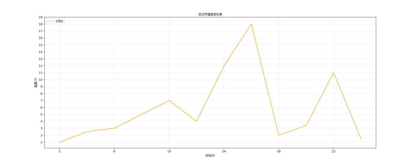
1. Draw line chart
1.1 basic use
# Introduce pyplot in matplotlib
from matplotlib import pyplot as plt
# Introduce font in matplotlib_ manager
from matplotlib import font_manager

# To generate x-axis data, it needs to be an iterative sequence
x = range(2, 24, 2)

# To generate y-axis data, it needs to be an iterative sequence
y = [1, 2, 12, 34, 2, 5,6,7,8,0,9.1]

# Set the width and height of the image to 20 and 8, and the pixels per inch to 90
plt.figure(figsize=(20, 8), dpi=90)

# Set Chinese font
font = font_manager.FontProperties(fname="C:\Windows\Fonts\msyh.ttc")

# Draw the image and label it, and specify the line color as orange
plt.plot(x, y, label="3 month", color="orange")

# Set the legend (it needs to be used in combination with the label attribute above)
plt.legend(loc="upper left", prop=font)

# Add grid
plt.grid(alpha=0.3)

# Add description information
plt.xlabel("time/h", fontproperties=font)
plt.ylabel("temperature/℃", fontproperties=font)
plt.title("Wuhan temperature change table", fontproperties=font)

# Display image
plt.show()
1.2 setting picture size and definition
# Set the width and height to 20 and 8, and 100 pixels per inch
plt.figure(figsize=(20, 8), dpi=100)
1.3 saving the generated image
# Save picture
plt.savefig('./demo.svg')
1.4 setting fonts
# Introduce font in matplotlib_ manager
from matplotlib import font_manager
# Set Chinese font
font = font_manager.FontProperties(fname="C:\Windows\Fonts\msyh.ttc")
1.5 add description information
# Add description information
plt.xlabel("time/h", fontproperties=font)
plt.ylabel("temperature/℃", fontproperties=font)
plt.title("Wuhan temperature change table", fontproperties=font)
1.6 setting legend
# Set Chinese font
font = font_manager.FontProperties(fname="C:\Windows\Fonts\msyh.ttc")
# Draw and label images
plt.plot(x, y, label="3 month")
# Set the legend (it needs to be used in combination with the label attribute above)
plt.legend(loc="upper left", prop=font)
1.7 setting grid
# Draw the grid of the image (conducive to observing the data)
plt.grid(alpha=0.3)
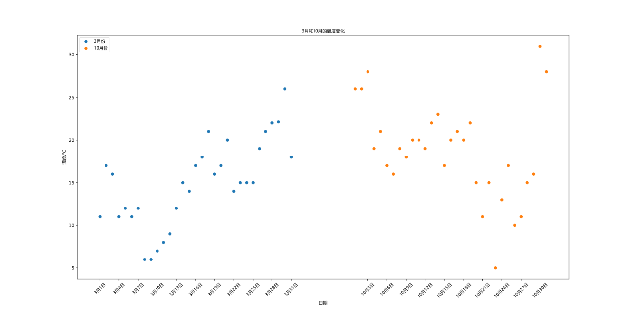
2. Draw scatter diagram
Draw the scatter diagram of temperature change in March and October
from matplotlib import pyplot as plt
from matplotlib import font_manager

# Daily temperature in March
y_3 = [11, 17, 16, 11, 12, 11, 12, 6, 6, 7, 8, 9, 12, 15, 14, 17, 18, 21, 16, 17, 20, 14, 15, 15, 15, 19, 21, 22, 22.12, 26, 18]
# Daily temperature in October
y_10 = [26, 26, 28, 19, 21, 17, 16, 19, 18, 20, 20, 19, 22, 23, 17, 20, 21, 20, 22, 15, 11, 15, 5, 13, 17, 10, 11, 15, 16, 31, 28]
# Set image size
plt.figure(figsize=(20, 8), dpi=80)

# Set font
font = font_manager.FontProperties(fname="C:\Windows\Fonts\msyh.ttc")

x_3 = range(1, 32)
x_10 = range(41, 72)

# Draw image
plt.scatter(x_3, y_3, label="3 month")
plt.scatter(x_10, y_10, label="10 month")

# Set legend
plt.legend(loc="upper left", prop=font)

# Set the scale of x
x_ticks = list(x_3) + list(x_10)
x_labels = ["3 month{}day".format(i) for i in x_3]
x_labels += ["10 month{}day".format(i - 40) for i in x_10]
plt.xticks(ticks=x_ticks[::3], labels=x_labels[::3], fontproperties=font, rotation=45)

# Add description
plt.xlabel("date/Month day", fontproperties=font)
plt.ylabel("temperature/℃", fontproperties=font)
plt.title("3 Table of temperature changes in October and October", fontproperties=font)
# Save the image
plt.savefig('./scatter.svg')

# Display image
plt.show()
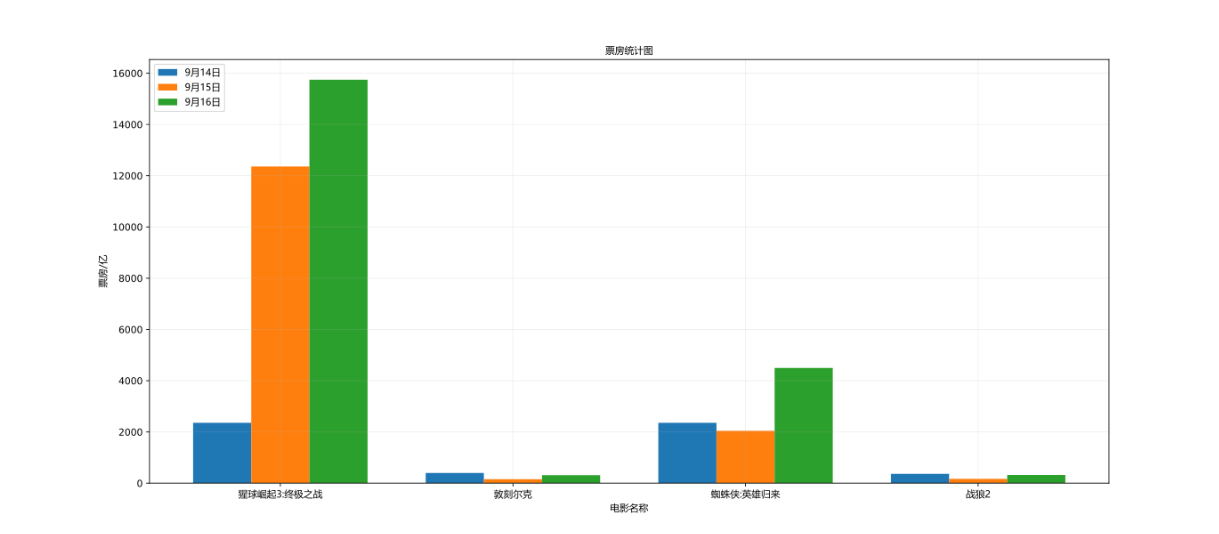
3. Draw bar chart
Draw the box office numbers of four popular films on September 14, September 15 and September 16 respectively
from matplotlib import pyplot as plt
from matplotlib import font_manager

# The names of the four films
a = ["The rise of the scarlet ball 3:The ultimate battle", "Dunkirk", "Spider-Man:Hero return", "Warwolf 2"]

# Box office of four films on the 14th
y_14 = [2358, 399, 2358, 362]
# Box office of four films on the 15th
y_15 = [12357, 156, 2045, 168]
# Box office of four films on the 16th
y_16 = [15746, 312, 4497, 319]

# Sets the size of the image
plt.figure(figsize=(20,9), dpi=80)

# Set Chinese font
font = font_manager.FontProperties(fname="C:\Windows\Fonts\msyh.ttc")

# Sets the width of the bar column uniformly
x_width = 0.25

# Generate x-axis data
x_14 = range(len(a))
# [0, 1, 2, 3]
x_15 = [i+x_width for i in x_14]
# [0.25, 1.25, 2.25, 3.25]
x_16 = [i+2*x_width for i in x_14]
# [0.5, 1.5, 2.5, 3.5]

# Draw image
plt.bar(x_14, y_14, width=x_width, label="9 May 14")
plt.bar(x_15, y_15, width=x_width, label="9 May 15")
plt.bar(x_16, y_16, width=x_width, label="9 June 16")

# Add legend (used in combination with the above label)
plt.legend(loc="upper left", prop=font)

# Sets the scale of the x-axis
plt.xticks(ticks=x_15, labels=a, fontproperties=font)

# Add description information
plt.title("Box office statistics", fontproperties=font)
plt.xlabel("Movie title", fontproperties=font)
plt.ylabel("box office/Hundred million", fontproperties=font)

# Adding a grid is helpful to observe the data
plt.grid(alpha=0.2)

# Save image
plt.savefig('./bar.svg')

plt.show()
4, Use of numpy
1. numpy basic usage
1.1 generate numpy array
# Three ways to generate numpy.ndarray
# Mode 1
t1 = np.array(range(10))
print(t1)
[0 1 2 3 4 5 6 7 8 9]
print(t1.dtype)
int32
# Mode II
t2 = np.array([1, 2, 3, 4, 5])
print(t2)
[1 2 3 4 5]
# Mode III
t3 = np.arange(2, 18, 2)
print(t3)
[ 2  4  6  8 10 12 14 16]
1.2 specify the data type of the generated array
# Specifies the data type of the generated array
t4 = np.array([1, 1, 0, 0, 1, 0], dtype=bool)
print(t4)
[ True  True False False  True False]
1.3 modify the data type of the array
# Modify the data type of the array
t5 = np.array([True, True, False, False, True, False])
t6 = t5.astype(dtype="int32")
print(t6)
[1 1 0 0 1 0]
1.4 specify the number of decimal places in the array
# Specifies the number of decimal places in the array
# Generate an array containing decimals. random.random() can generate decimals of [0,1]
t7 = np.array([random.random() for i in range(10)])
print(t7)
[0.13195263 0.65366942 0.33832589 0.84553949 0.0674462  0.9550536 0.91240518 0.50317671 0.28403965 0.98534765]
# Keep two decimal places
t8 = t7.round(2)
print(t8)
[0.13 0.65 0.34 0.85 0.07 0.96 0.91 0.5  0.28 0.99]
1.5 viewing and modifying array shapes
# View the shape of an array
t9 = np.array(range(12))
print(t9)
[ 0  1  2  3  4  5  6  7  8  9 10 11]
# When the array has only one row of data, the shape value represents the number of array elements
print(t9.shape)
(12,)

# Modify the shape of the array (change to a two-dimensional array with 3 rows and 4 columns)
t10 = t9.reshape((3, 4))
print(t10)
[[ 0  1  2  3]
 [ 4  5  6  7]
 [ 8  9 10 11]]
# When the array is a two-dimensional array, the shape value represents the number of rows and columns
print(t10.shape)
(3, 4)
2. Calculation of numpy array
2.1 calculation of arrays and numbers
Taking advantage of its broadcasting, the number will be converted into an array of corresponding dimensions for calculation.
# Calculation of arrays and numbers
a = np.array([1, 2, 3, 4])
print(f"The result of addition is:{a + 1}")
[2 3 4 5]
print(f"The result of multiplication is:{a * 2}")
[2 4 6 8]
print(f"The result of the power is:{a ** 2}")
[ 1  4  9 16]
2.2 array and array calculation
# Array and array calculation
a = np.array([1, 2, 3, 4])
b = np.array([2, 3, 4, 5])
print(f"The result of array addition is:{a + b}")
[3 5 7 9]
print(f"The result of array multiplication is:{a * b}")
[ 2  6 12 20]
print(f"The result of array power is:{a ** b}")
[   1    8   81 1024]
2.3 transpose of array (matrix)
# Transpose of array (matrix)
print(c.T)
3. numpy reads local data
csv file for testing (demo.csv)
7426393,78240,13548,7054
94203,2651,1309,0
7426393,78240,13548,7054
94203,2651,1309,0
142819,13119,151,114115
80028,65729,1529,3598
40592,5019,57,490
142819,13119,151,11411
580028,65729,1529,35984
0592,5019,57,490
317696,9449,135,4644
79291,23935,638,1941
317696,9449,135,46447
9291,23935,638,1941
10532409,384841,7547,238496
5453,2761,33,223
751743,42272,358,325011
read file
# Path of local csv file
file_path = "./demo.csv"

# Read csv file
# dtype means to convert the read characters into the corresponding data type. The default is float type
# delimiter indicates what separator is used to extract content. By default, it is by space
data = np.loadtxt(file_path, delimiter=",", dtype=int)

# Type of output data
print(type(data))
<class 'numpy.ndarray'>
# Output read data
print(data)
[[ 7426393    78240    13548     7054]
 [   94203     2651     1309        0]
 [ 7426393    78240    13548     7054]
 [   94203     2651     1309        0]
 [  142819    13119      151   114115]]
4. numpy index and slicing
4.1 numpy index
# Generate a two-dimensional array of 5 rows and 8 columns
data = np.arange(10, 25).reshape((3, 5))

# Output 2D array
print(data)
[[10 11 12 13 14]
 [15 16 17 18 19]
 [20 21 22 23 24]]

# First row of output array
print(data[0])
[10 11 12 13 14]
# Output the data of the first row and the second column of the array
print(data[0][1])
11
4.2 numpy slice
# Generate a two-dimensional array of 5 rows and 8 columns
data = np.arange(10, 25).reshape((3, 5))

# Output 2D array
print(data)
[[10 11 12 13 14]
 [15 16 17 18 19]
 [20 21 22 23 24]]

# When slicing, the row before "," represents the row, and the column after "," represents the column

# Output the second and third columns in the first row of the array
print(data[0, 1:3])
[11 12]
# Output the second column of the array
print(data[:, 1])
[11 16 21]
# Output the second and third columns of the array
print(data[:, 1:3])
[[11 12]
 [16 17]
 [21 22]]
# Take the discontinuous line, the first line and the third line
print(data[[0, 2]])
[[10 11 12 13 14]
 [20 21 22 23 24]]
# Take the discontinuous columns, the first and third columns and the fourth column
print(data[:, [0, 2, 3]])
[[10 12 13]
 [15 17 18]
 [20 22 23]]
5. numpy common methods
5.1 numpy ternary operator
# Generate a two-dimensional array of 5 rows and 8 columns
data = np.arange(10, 25).reshape((3, 5))
# Output 2D array
print(data)
[[10 11 12 13 14]
 [15 16 17 18 19]
 [20 21 22 23 24]]

# Ternary operator: if each data in data is less than 20, it will be set to 0; otherwise, it will be set to 20
t = np.where(data < 20, 0, 20)
print(t)
[[ 0  0  0  0  0]
 [ 0  0  0  0  0]
 [20 20 20 20 20]]
5.2 array splicing
# Prepare array data
# Generate an array of 3 rows and 4 columns
t1 = np.arange(12).reshape((3, 4))
print(t1)
[[ 0  1  2  3]
 [ 4  5  6  7]
 [ 8  9 10 11]]
# Generate an array of 3 rows and 2 columns
t2 = np.arange(6).reshape((3, 2))
print(t2)
[[0 1]
 [2 3]
 [4 5]]
# Generate an array of 1 row and 4 columns
t3 = np.arange(4).reshape((1, 4))
print(t3)
[[0 1 2 3]]

# Array splicing
# Horizontal splicing
t4 = np.hstack((t1, t2))
print(t4)
[[ 0  1  2  3  0  1]
 [ 4  5  6  7  2  3]
 [ 8  9 10 11  4  5]]
# Vertical splicing
t5 = np.vstack((t1, t3))
print(t5)
[[ 0  1  2  3]
 [ 4  5  6  7]
 [ 8  9 10 11]
 [ 0  1  2  3]]
5.3 row column exchange of array
# Generate an array of 3 rows and 4 columns
t1 = np.arange(12).reshape((3, 4))
print(t1)
[[ 0  1  2  3]
 [ 4  5  6  7]
 [ 8  9 10 11]]

# Row exchange and column exchange of arrays
# Line swap (swap lines 1 and 3)
t1[[0, 2], :] = t1[[2, 0], :]
print(t1)
[[ 8  9 10 11]
 [ 4  5  6  7]
 [ 0  1  2  3]]
# Column exchange (exchange columns 2 and 4)
t1[:, [1, 3]] = t1[:, [3, 1]]
print(t1)
[[ 0  3  2  1]
 [ 4  7  6  5]
 [ 8 11 10  9]]
5.4 generating identity matrix
import numpy as np
# Generate 3 * 3 identity matrix
t1 = np.eye(3)
print(t1)
[[1. 0. 0.]
 [0. 1. 0.]
 [0. 0. 1.]]
# Convert the data in t11 to type int
t2 = t1.astype(int)
print(t2)
[[1 0 0]
 [0 1 0]
 [0 0 1]]
5, Use of pandas
1. Series objects
The Series object is one-dimensional and has an index and a corresponding value.
# Pass in a list to generate a Series object
ps1 = pd.Series([1, 2, 3, 4, 5])
print(ps1)
0    1
1    2
2    3
3    4
4    5
dtype: int64
# Pass in a range object to generate a Series object
ps2 = pd.Series(range(5))
print(ps2)
0    0
1    1
2    2
3    3
4    4
dtype: int64
# Pass in a dict dictionary object whose key corresponds to the index of the generated Series object
data = {"name": "Lu Sheng Liu", "age": 10}
print(pd.Series(data))
name    Lu Sheng Liu
age      10
dtype: object
# Specifies the index of the index
ps3 = pd.Series([1, 2, 3, 4], index=list("abcd"))
print(ps3)
a    1
b    2
c    3
d    4
dtype: int64
# Modify the type of data
ps4 = ps3.astype(float)
print(ps4)
a    1.0
b    2.0
c    3.0
d    4.0
dtype: float64
# View indexes and values of Series objects
print(ps4.index)
print(ps4.values)
Index(['a', 'b', 'c', 'd'], dtype='object')
[1. 2. 3. 4.]
# Sum
print(ps4.sum())
10.0
2. DataFrame object
The DataFrame object is a two-dimensional container of Series, which has row index and column index.
# Pass in a 3 * 3 numpy array as a parameter to generate a DataFrame object
df1 = pd.DataFrame(np.arange(9).reshape((3, 3)))
print(df1)
   0  1  2
0  0  1  2
1  3  4  5
2  6  7  8

# Specifies the values for the row and column indexes
df2 = pd.DataFrame(np.arange(9).reshape((3, 3)), index=list("abc"), columns=list("DEF"))
print(df2)
   D  E  F
a  0  1  2
b  3  4  5
c  6  7  8
3. Slicing and indexing of dataframe
loc [row, column]: applicable to DataFrame object with specified index alias.
iloc [row, column]: applicable to DataFrame objects with index numbers.
# Pass in a 3 * 3 numpy array as a parameter to generate a DataFrame object
df1 = pd.DataFrame(np.arange(9).reshape((3, 3)))
print(df1)
   0  1  2
0  0  1  2
1  3  4  5
2  6  7  8
# Specifies the values for the row and column indexes
df2 = pd.DataFrame(np.arange(9).reshape((3, 3)), index=list("abc"), columns=list("DEF"))
print(df2)
   D  E  F
a  0  1  2
b  3  4  5
c  6  7  8

# Use of loc
# Get all the values with column index E and return a Series object
ps2 = df2['E']
print(ps2)
a    1
b    4
c    7
Name: E, dtype: int32

# Gets the value with row index a and column index E
print(df2.loc["a", "E"])
1

# Get the values with row index a and column index D and E, and return the Series object
print(df2.loc["a", ["D", "E"]])
D    0
E    1
Name: a, dtype: int32

# Get the values with row indexes a and b and column indexes D and E, and return the DataFrame object
print(df2.loc[["a", "b"], ["D", "E"]])
   D  E
a  0  1
b  3  4

# Use of iloc
# Get all the values of the first column and return a Series object
ps1 = df1[0]
print(ps1)
0    0
1    3
2    6
Name: 0, dtype: int32

# Get the value of row 1 and column 2
print(df1.iloc[0, 1])
1

# Get the values of columns 1 and 2 in Row 2, and return a Series object
print(df1.iloc[1, [0, 1]])
0    3
1    4
Name: 1, dtype: int32
4. Read external data
data.csv file
Name,Age,Number,Identity
 Zhang San,20,13334257846,graduate student
 Li Si,21,18875413624,undergraduate
 Wang Wu,25,14258796412,Doctor
 Zhao Liu,21,13334257846,undergraduate
 Lao Wang,28,14235648752,Doctor
 Xiaomei,16,12347859548,undergraduate
 Zhang San,22,15742687942,graduate student
# Read csv file
df = pd.read_csv("data.csv")
# View everything
print(df)

# View the contents of the first three lines
print(df.head(3))
  Name  Age       Number Identity
0   Zhang San 20 13334257846      graduate student
1   Li Si 21 18875413624      undergraduate
2   Wang Wu 25 14258796412      Doctor

# View read details
print(df.info())
<class 'pandas.core.frame.DataFrame'>
RangeIndex: 7 entries, 0 to 6
Data columns (total 4 columns):
 #   Column    Non-Null Count  Dtype
---  ------    --------------  -----
 0   Name      7 non-null      object
 1   Age       7 non-null      int64
 2   Number    7 non-null      int64
 3   Identity  7 non-null      object
dtypes: int64(2), object(2)
memory usage: 352.0+ bytes
None

# View the description information of the content (including mean value, variance, minimum value, maximum value, etc.) and only count numerical data
print(df.describe())
             Age        Number
count   7.000000  7.000000e+00
mean   21.857143  1.458985e+10
std     3.804759  2.164474e+09
min    16.000000  1.234786e+10
25%    20.500000  1.333426e+10
50%    21.000000  1.423565e+10
75%    23.500000  1.500074e+10
max    28.000000  1.887541e+10
5. Common data processing methods
Data use the data read above
# View the description information of the content (including mean value, variance, minimum value, maximum value, etc.) and only count numerical data
print(df.describe())
             Age        Number
count   7.000000  7.000000e+00
mean   21.857143  1.458985e+10
std     3.804759  2.164474e+09
min    16.000000  1.234786e+10
25%    20.500000  1.333426e+10
50%    21.000000  1.423565e+10
75%    23.500000  1.500074e+10
max    28.000000  1.887541e+10

# View the average value of the Age column
print(df['Age'].mean())
21.857142857142858

# View variance of Age column
print(df['Age'].std())
3.8047589248453675

"""
   XXX.str.xxx()There are other ways:
       -cat(And specified characters)
       -split((separated by specified string)
       -rsplit(and split The usage is the same, except that it is separated from right to left by default)
       -zfill(Fill, can only be 0, fill from the left)
       -contains(Determines whether the string contains the specified substring, and returns yes bool (type)
       More reference blog https://blog.csdn.net/weixin_43750377/article/details/107979607
"""
# Treat each value of the Name column as a string, cut the string according to the specified format to generate a list, and the final result returns a Series object
temp1 = df['Name'].str.split("")
print(temp1)
0    [, Zhang, three, ]
1    [, Lee, four, ]
2    [, king, five, ]
3    [, Zhao, six, ]
4    [, old, king, ]
5    [, Small, beautiful, ]
6    [, Zhang, three, ]
Name: Name, dtype: object

# Treat each value of the Name column as a string, cut the string according to the specified format, generate a list, and convert all the generated list values into a large list
list2 = df['Name'].str.split("").tolist()
print(list2)
[['', 'Zhang', 'three', ''], ['', 'Lee', 'four', ''], ['', 'king', 'five', ''], ['', 'Zhao', 'six', ''], ['', 'old', 'king', ''], ['', 'Small', 'beautiful', ''], ['', 'Zhang', 'three', '']]

# Treat each value of the Name column as a string and judge whether the string contains sheets. If yes, it returns True, otherwise it returns False, and the final result returns a Series object
print(df['Name'].str.contains('Zhang'))
0    False
1    False
2    False
3    False
4    False
5    False
6    False

# Remove duplicate elements and return the ndarray object
print(df['Name'].unique())
['Zhang San' 'Li Si' 'Wang Wu' 'Zhao Liu' 'Lao Wang' 'Xiaomei']