Introduction to pytorch
The article is only used to record your own learning. If there is infringement, delete it immediately
Some good websites
https://github.com/jcjohnson/pytorch-examples Some small projects of pytorch
https://pytorch.org/tutorials/ pytorch official tutorial
Fastai
Michael Nielsen's "Neural Network and Deep Learning" is some derivation of mathematical principles, but it is not necessary to learn pytorch
English online: http://neuralnetworksanddeeplearning.com/about.html
Chinese version:
Convex optimization by Stephen Boyd and Lieven Vandenberghe
3lue1brown video explains knowledge about mathematics and so on https://space.bilibili.com/88461692
pytorch official tutorial
Here are some lessons from pytorch's official tutorials
https://pytorch.org/tutorials/ See the original text below is some of my own translation and learning
LEARN THE BASICS
Authors: Suraj Subramanian, Seth Juarez, Cassie Breviu, Dmitry Soshnikov, Ari Bornstein
Most machine learning workflows involve processing data, creating models, optimizing model parameters, and saving trained models. Next, let's follow the tutorial to learn about pytorch, and then experiment on the minst dataset
There are two ways to learn. One is to run the sample code in the notebook on the cloud
Each section has a "Run in Microsoft Learn" link at the top
The other is to deploy the environment locally
QUICKSTART
PyTorch has two statements for processing data
torch.utils.data.DataLoader and torch.utils.data.Dataset
The Dataset stores samples and their corresponding labels
DataLoader encapsulates the dataset as an iterable (iterator interface)
import torch
from torch import nn
from torch.utils.data import DataLoader
from torchvision import datasets
from torchvision.transforms import ToTensor, Lambda, Compose
import matplotlib.pyplot as plt
PyTorch provides domain specific libraries such as TorchText, TorchVision, and TorchAudio, all of which contain data sets. In this tutorial, we will use the TorchVision dataset.
torchvision.datasets module contains many datasets, such as coco and cifra
Each TorchVision dataset contains two parameters: transform and target_transform, which is used to modify samples and labels respectively.
example
# Download training data from open datasets.
training_data = datasets.FashionMNIST(
    root="data",
    train=True,
    download=True,
    transform=ToTensor(),
)

# Download test data from open datasets.
test_data = datasets.FashionMNIST(
    root="data",
    train=False,
    download=True,
    transform=ToTensor(),
)
We pass the dataset as a parameter to the DataLoader. This wraps an iterable on our dataset and supports automatic batch processing, sampling, mixing and multi process data loading. Here, we define 64 batch sizes, that is, each element in the dataloader iterable will return a batch of 64 features and labels.
batch_size = 64

# Create data loaders.
train_dataloader = DataLoader(training_data, batch_size=batch_size)
test_dataloader = DataLoader(test_data, batch_size=batch_size)

for X, y in test_dataloader:
    print("Shape of X [N, C, H, W]: ", X.shape)
    print("Shape of y: ", y.shape, y.dtype)
    break
Note: from the above, we can learn the logic of pytorch reading the data set, and understand the logic of pytorch processing the data set (that is, it becomes an iterable). Next, consider how to create a model
Creating Models
In order to define the neural network in PyTorch, we created a class inherited from nn.Module. We are_ init__ Function, and specify how the data will pass through the network in the forward function. To speed up the operation in the neural network, we move it to the GPU (if available).
# Get cpu or gpu device for training.
device = "cuda" if torch.cuda.is_available() else "cpu"
print(f"Using {device} device")

# Define model
class NeuralNetwork(nn.Module):
    def __init__(self):
        super(NeuralNetwork, self).__init__()
        self.flatten = nn.Flatten()
        self.linear_relu_stack = nn.Sequential(
            nn.Linear(28*28, 512),
            nn.ReLU(),
            nn.Linear(512, 512),
            nn.ReLU(),
            nn.Linear(512, 10)
        )

    def forward(self, x):
        x = self.flatten(x)
        logits = self.linear_relu_stack(x)
        return logits

model = NeuralNetwork().to(device)
print(model)
The interpretation of this network structure will be left behind
Optimizing the Model Parameters
After the network structure is determined, we need to consider how to train the network parameters we need. Therefore, we need to define loss function and optimizer
loss_fn = nn.CrossEntropyLoss()
optimizer = torch.optim.SGD(model.parameters(), lr=1e-3)
First sentence: cross entropy loss
Second sentence SGD optimizer
In a single training cycle, the model predicts the training data set (batch input), and back propagates the prediction error to adjust the model parameters.
def train(dataloader, model, loss_fn, optimizer):
    size = len(dataloader.dataset)
    model.train()
    for batch, (X, y) in enumerate(dataloader):
        X, y = X.to(device), y.to(device)

        # Compute prediction error
        pred = model(X)# The output is the predicted output
        loss = loss_fn(pred, y)# Calculate loss

        # Backpropagation Algorithm
        optimizer.zero_grad()# Gradient zero
        loss.backward()
        optimizer.step()

        if batch % 100 == 0:
            loss, current = loss.item(), batch * len(X)
            print(f"loss: {loss:>7f}  [{current:>5d}/{size:>5d}]")
Take a closer look at the specific code, cooperate with the previous model, and explain it in detail later in combination with the comments written
def test(dataloader, model, loss_fn):
    size = len(dataloader.dataset)
    num_batches = len(dataloader)
    model.eval()
    test_loss, correct = 0, 0
    with torch.no_grad():
        for X, y in dataloader:
            X, y = X.to(device), y.to(device)
            pred = model(X)
            test_loss += loss_fn(pred, y).item()
            correct += (pred.argmax(1) == y).type(torch.float).sum().item()
    test_loss /= num_batches
    correct /= size
    print(f"Test Error: \n Accuracy: {(100*correct):>0.1f}%, Avg loss: {test_loss:>8f} \n")
The training process is carried out in multiple iterations (epoch). In each epoch, the model learns parameters to make better predictions. We print the accuracy and loss of the model in each epoch; We want to see the accuracy decrease with the increase of each epoch.
epochs = 5
for t in range(epochs):
    print(f"Epoch {t+1}\n-------------------------------")
    train(train_dataloader, model, loss_fn, optimizer)
    test(test_dataloader, model, loss_fn)
print("Done!")
saving Models and loading
torch.save(model.state_dict(), "model.pth")
print("Saved PyTorch Model State to model.pth")
Save model operation
model = NeuralNetwork()
model.load_state_dict(torch.load("model.pth"))
This concludes the first chapter on reading models. The next chapter introduces tensors
Tensors
This chapter mainly introduces the concept of tensor
Tensors are a specialized data structure that are very similar to arrays and matrices
Tensor is a special data structure, which is very similar to array and matrix. It can be understood as the storage structure in pytorch. We use tensors to encode the input and output of the model and the parameters of the model.
Tensors are similar to NumPy's ndarray, except that they can run on GPU or other hardware accelerators. Tensor and NumPy arrays can usually share the same underlying memory without copying data
import torch
import numpy as np
Initializing a Tensor / creating a tensor
Import tensor from data (matrix form)
data = [[1, 2],[3, 4]]
x_data = torch.tensor(data)
Import tensor from numpy array
np_array = np.array(data)
x_np = torch.from_numpy(np_array)
Import from another tensor (unless explicitly overridden, the new tensor retains the properties (shape, data type) of the parameter tensor)
x_ones = torch.ones_like(x_data)
# Retain the properties of x_data
print(f"Ones Tensor: \n {x_ones} \n")

x_rand = torch.rand_like(x_data, dtype=torch.float)
# overrides the datatype of x_data
print(f"Random Tensor: \n {x_rand} \n")
Out:
Ones Tensor:
 tensor([[1, 1],
        [1, 1]])

Random Tensor:
 tensor([[0.3277, 0.7579],
        [0.1860, 0.8509]])
Define the size shape of the tensor and fill it with constant or random values
shape = (2,3,)
rand_tensor = torch.rand(shape)
ones_tensor = torch.ones(shape)
zeros_tensor = torch.zeros(shape)

print(f"Random Tensor: \n {rand_tensor} \n")
print(f"Ones Tensor: \n {ones_tensor} \n")
print(f"Zeros Tensor: \n {zeros_tensor}")
Out:
Random Tensor:
 tensor([[0.2882, 0.0322, 0.4411],
        [0.5961, 0.6428, 0.1681]])

Ones Tensor:
 tensor([[1., 1., 1.],
        [1., 1., 1.]])

Zeros Tensor:
 tensor([[0., 0., 0.],
        [0., 0., 0.]])
Some properties or interfaces available to tensor
shape dtype device
tensor = torch.rand(3,4)

print(f"Shape of tensor: {tensor.shape}")
print(f"Datatype of tensor: {tensor.dtype}")
print(f"Device tensor is stored on: {tensor.device}")
Out:
Shape of tensor: torch.Size([3, 4])
Datatype of tensor: torch.float32
Device tensor is stored on: cpu
Operation of tensor
The syntax is similar to that of python or matlab, which is easy to understand
tensor = torch.ones(4, 4)
print('First row: ', tensor[0])
print('First column: ', tensor[:, 0])
print('Last column:', tensor[..., -1])
tensor[:,1] = 0
print(tensor)
Out:
First row:  tensor([1., 1., 1., 1.])
First column:  tensor([1., 1., 1., 1.])
Last column: tensor([1., 1., 1., 1.])
tensor([[1., 0., 1., 1.],
        [1., 0., 1., 1.],
        [1., 0., 1., 1.],
        [1., 0., 1., 1.]])
Connection operation
t1 = torch.cat([tensor, tensor, tensor], dim=1)
print(t1)
Out:
tensor([[1., 0., 1., 1., 1., 0., 1., 1., 1., 0., 1., 1.],
        [1., 0., 1., 1., 1., 0., 1., 1., 1., 0., 1., 1.],
        [1., 0., 1., 1., 1., 0., 1., 1., 1., 0., 1., 1.],
        [1., 0., 1., 1., 1., 0., 1., 1., 1., 0., 1., 1.]])
arithmetic operation
# This computes the matrix multiplication between two tensors. y1, y2, y3 will have the same value
#tensor matrix multiplication, y1, y2, y3 are all matrix multiplication results
y1 = tensor @ tensor.T
y2 = tensor.matmul(tensor.T)

y3 = torch.rand_like(tensor)
torch.matmul(tensor, tensor.T, out=y3)


# This computes the element-wise product. z1, z2, z3 will have the same value
# Tensor point multiplication tensor element by element product each other
z1 = tensor * tensor
z2 = tensor.mul(tensor)

z3 = torch.rand_like(tensor)
torch.mul(tensor, tensor, out=z3)
Single element tensor: if you have a single element tensor, for example, by aggregating all the values of the tensor into one value, you can convert it to Python values using item()
agg = tensor.sum()
agg_item = agg.item()
print(agg_item, type(agg_item))
Out:
12.0 <class 'float'>
In place operations operations that store results in operands are called in place operations. They are represented by the suffix "". For example:: x.copy_(y), x.t_(), will change x
print(tensor, "\n")
tensor.add_(5)
print(tensor)
Out:
tensor([[1., 0., 1., 1.],
        [1., 0., 1., 1.],
        [1., 0., 1., 1.],
        [1., 0., 1., 1.]])

tensor([[6., 5., 6., 6.],
        [6., 5., 6., 6.],
        [6., 5., 6., 6.],
        [6., 5., 6., 6.]])
Detailed explanation of datasets & dataloaders
The code that handles data samples can become messy and difficult to maintain; we ideally want our Dataset code to be separated from our model training code for better readability and modularity. PyTorch provides two data primitives: torch.utils.data.DataLoader and torch.utils.data.Dataset, which allow you to use preloaded datasets and yourself The Dataset stores samples and their corresponding tags, and the DataLoader wraps an iteratable object around the Dataset to easily access the samples.
The PyTorch domain library provides many preloaded datasets (such as FashionMNIST), which are subclasses of torch.utils.data.Dataset and implement data specific functions. They can be used for prototyping and benchmarking your model.
Relevant parameters of Load Dataset FashionMNIST Dataset take as an example
-
root is the path where the train/test data is stored, in short, the address, the location where the data set is placed or to be downloaded
-
Train specific training or test dataset
-
download=True downloads the data from the internet if it's not available at root
-
transform and target_transform specify the feature and label transformations specify what transform to use
import torch
from torch.utils.data import Dataset
from torchvision import datasets
from torchvision.transforms import ToTensor
import matplotlib.pyplot as plt


training_data = datasets.FashionMNIST(
    root="data",
    train=True,
    download=True,
    transform=ToTensor()
)

test_data = datasets.FashionMNIST(
    root="data",
    train=False,
    download=True,
    transform=ToTensor()
)
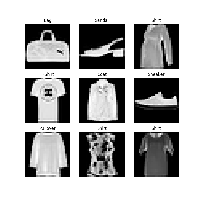
Visual dataset
We can manually index the dataset like a list: training_data[index]. We use matplotlib to visualize some samples in the training data.
labels_map = {
    0: "T-Shirt",
    1: "Trouser",
    2: "Pullover",
    3: "Dress",
    4: "Coat",
    5: "Sandal",
    6: "Shirt",
    7: "Sneaker",
    8: "Bag",
    9: "Ankle Boot",
}
figure = plt.figure(figsize=(8, 8))
cols, rows = 3, 3
for i in range(1, cols * rows + 1):
    sample_idx = torch.randint(len(training_data), size=(1,)).item()
    img, label = training_data[sample_idx]
    figure.add_subplot(rows, cols, i)
    plt.title(labels_map[label])
    plt.axis("off")
    plt.imshow(img.squeeze(), cmap="gray")
plt.show()
Create a custom dataset
A custom dataset must contain:
: __init__, __len__, and __getitem__.
Three functions
For example, take the FashionMNIST dataset as an example
Images are stored in the directory img_ In dir, their labels are stored separately in the CSV file annotations_file.
import os
import pandas as pd
from torchvision.io import read_image

class CustomImageDataset(Dataset):
    def __init__(self, annotations_file, img_dir, transform=None, target_transform=None):
        self.img_labels = pd.read_csv(annotations_file)
        self.img_dir = img_dir
        self.transform = transform
        self.target_transform = target_transform

    def __len__(self):
        return len(self.img_labels)

    def __getitem__(self, idx):
        img_path = os.path.join(self.img_dir, self.img_labels.iloc[idx, 0])
        image = read_image(img_path)
        label = self.img_labels.iloc[idx, 1]
        if self.transform:
            image = self.transform(image)
        if self.target_transform:
            label = self.target_transform(label)
        return image, label
__ init__ function
__ init__ The function runs once when instantiating the Dataset object. We initialize a directory that contains images, annotation files, and two transformations
labels.csv file, for example
tshirt1.jpg, 0
tshirt2.jpg, 0
......
ankleboot999.jpg, 9
def __init__(self, annotations_file, img_dir, transform=None, target_transform=None):
    self.img_labels = pd.read_csv(annotations_file, names=['file_name', 'label'])
    self.img_dir = img_dir
    self.transform = transform
    self.target_transform = target_transform
__ len__ Function returns the number of samples in our dataset.
def __len__(self):
    return len(self.img_labels)
__ getitem__ Function loads and returns a sample from the dataset of the given index idx. Based on the index, it identifies the position of the image on the disk and uses read_image converts it to a tensor from self.img_ Retrieve the corresponding tags from the csv data in labels, call their conversion functions (if applicable), and return the corresponding tags in tensor images and tuples.
def __getitem__(self, idx):
    img_path = os.path.join(self.img_dir, self.img_labels.iloc[idx, 0])
    image = read_image(img_path)
    label = self.img_labels.iloc[idx, 1]
    if self.transform:
        image = self.transform(image)
    if self.target_transform:
        label = self.target_transform(label)
    return image, label
Using data set to transfer data for training
The dataset retrieves the features of our dataset and marks one sample at a time. When training models, we usually want to transfer samples in the form of "small batch", reshuffle the data in each period to reduce over fitting of the model, and use Python's multiprocessing to speed up data retrieval.
DataLoader is an iterator that abstracts this complexity for us in a simple API.
from torch.utils.data import DataLoader

train_dataloader = DataLoader(training_data, batch_size=64, shuffle=True)
test_dataloader = DataLoader(test_data, batch_size=64, shuffle=True)
Traverse DataLoader
We have loaded the dataset into the DataLoader and can traverse the dataset as needed. Each iteration below will return a batch of trains_ Features and train_labels (including batch_size=64 features and labels respectively). Because we specify shuffle=True, the data will be disrupted after we traverse all batches
# Display image and label.
train_features, train_labels = next(iter(train_dataloader))
print(f"Feature batch shape: {train_features.size()}")
print(f"Labels batch shape: {train_labels.size()}")
img = train_features[0].squeeze()
label = train_labels[0]
plt.imshow(img, cmap="gray")
plt.show()
print(f"Label: {label}")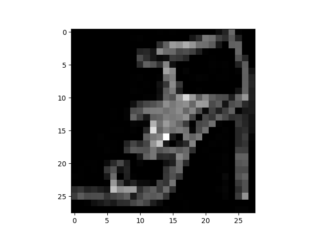
Out:
Feature batch shape: torch.Size([64, 1, 28, 28])
Labels batch shape: torch.Size([64])
Label: 5
Introduction to TRANSFORMS
In short, transform is to operate data to make it suitable for our network operation, that is, the data does not always appear in the final processing form required for training machine learning algorithms. We use transformation to manipulate the data and make it suitable for training.
All TorchVision datasets have two parameters - transform is used to modify the feature, target_ Transforms are used to modify tags -- they accept callable objects that contain transformation logic. The torchvision.transforms module provides several common transformations out of the box.
Fortunately, pytorch integrates a good transform function, so we don't have to bother writing new functions
import torch
from torchvision import datasets
from torchvision.transforms import ToTensor, Lambda

ds = datasets.FashionMNIST(
    root="data",
    train=True,
    download=True,
    transform=ToTensor(),
    target_transform=Lambda(lambda y: torch.zeros(10, dtype=torch.float).scatter_(0, torch.tensor(y), value=1))
)
ToTensor()
ToTensor() converts a PIL image or NumPy ndarray to FloatTensor. And the pixel intensity value of the image is scaled within the range of [0,1.]
Build the network
Neural networks consist of layers / modules that perform operations on data. The torch.nn namespace provides all the building blocks needed to build your own neural network. Each module in PyTorch is a subclass of nn.Module. Neural network is a module itself, which is composed of other modules (layers). This nested structure allows you to easily build and manage complex architectures.
import os
import torch
from torch import nn
from torch.utils.data import DataLoader
from torchvision import datasets, transforms
Select the device cpu or gpu to use
device = 'cuda' if torch.cuda.is_available() else 'cpu'
print(f'Using {device} device')
Define class
We define our neural network by inheriting nn.Module and initialize the neural network layer in init. Each NN. Module subclass implements the operation on the input data in the forward method.
class NeuralNetwork(nn.Module):
    def __init__(self):
        super(NeuralNetwork, self).__init__()
        self.flatten = nn.Flatten()
        self.linear_relu_stack = nn.Sequential(
            nn.Linear(28*28, 512),
            nn.ReLU(),
            nn.Linear(512, 512),
            nn.ReLU(),
            nn.Linear(512, 10),
        )

    def forward(self, x):
        x = self.flatten(x)
        logits = self.linear_relu_stack(x)
        return logits
model = NeuralNetwork().to(device)
print(model)
Network structure: linear layer + relu layer + linear layer + relu layer to linear layer
Out:
NeuralNetwork(
  (flatten): Flatten(start_dim=1, end_dim=-1)
  (linear_relu_stack): Sequential(
    (0): Linear(in_features=784, out_features=512, bias=True)
    (1): ReLU()
    (2): Linear(in_features=512, out_features=512, bias=True)
    (3): ReLU()
    (4): Linear(in_features=512, out_features=10, bias=True)
  )
)
In order to use the model, we pass the input data to it. This will perform forwarding of the model, as well as some background operations. Do not directly call model.forward()!
Calling the model on the input returns a 10 dimensional tensor containing the original predicted value of each class. We obtain the prediction probability by passing it to the instance of nn.Softmax module.
X = torch.rand(1, 28, 28, device=device)
logits = model(X)
pred_probab = nn.Softmax(dim=1)(logits)
y_pred = pred_probab.argmax(1)
print(f"Predicted class: {y_pred}")
The role of each module can be seen in combination with the 3bulue1brown MLP principle written in the previous article
Take a small batch sample consisting of three images with a size of 28x28 and see what happens when we transfer it over the network.
input_image = torch.rand(3,28,28)
print(input_image.size())
Out:
torch.Size([3, 28, 28])
nn.Flatten
We initialize the [nn.Flatten] layer to convert each 2D 28x28 image into a continuous array of 784 pixel values (the small batch dimension (when dim=0) is maintained).
flatten = nn.Flatten()
flat_image = flatten(input_image)
print(flat_image.size())
Out:
torch.Size([3, 784])
nn.Linear
nn.Linear is a module that uses its stored weights and deviations to apply a linear transformation to the input.
layer1 = nn.Linear(in_features=28*28, out_features=20)
hidden1 = layer1(flat_image)
print(hidden1.size())
Out:
torch.Size([3, 20])
nn.ReLU
nn.ReLU nonlinear activation is the reason for creating a complex mapping between the input and output of the model. They are applied after linear transformation to introduce nonlinearity and help neural networks learn a variety of phenomena.
In this model, we use [nn.ReLU] between our linear layers, but there are other activations to introduce nonlinearity into your model.
print(f"Before ReLU: {hidden1}\n\n")
hidden1 = nn.ReLU()(hidden1)
print(f"After ReLU: {hidden1}")
Out:
Before ReLU: tensor([[-0.5059,  0.0748, -0.3764,  0.2702, -0.5308,  0.1879, -0.1396, -0.1809,
         -0.0651,  0.1935,  0.8745,  0.3594, -0.0366,  0.4182, -0.4431,  0.2117,
         -0.2114, -0.0045, -0.2030, -0.5195],
        [-0.6142, -0.0293,  0.1397,  0.2526, -0.2365,  0.2625, -0.2154, -0.1611,
         -0.0842, -0.0181,  0.8274,  0.0739,  0.2244,  0.3389, -0.2915,  0.0280,
          0.0083, -0.3871, -0.3059, -0.0009],
        [-0.4356,  0.0336,  0.0208,  0.5318, -0.4322,  0.2168,  0.1233, -0.2511,
         -0.0217, -0.0147,  0.6722,  0.0350,  0.0696,  0.6650, -0.3241,  0.0591,
         -0.1873,  0.0044, -0.1151, -0.3288]], grad_fn=<AddmmBackward0>)


After ReLU: tensor([[0.0000, 0.0748, 0.0000, 0.2702, 0.0000, 0.1879, 0.0000, 0.0000, 0.0000,
         0.1935, 0.8745, 0.3594, 0.0000, 0.4182, 0.0000, 0.2117, 0.0000, 0.0000,
         0.0000, 0.0000],
        [0.0000, 0.0000, 0.1397, 0.2526, 0.0000, 0.2625, 0.0000, 0.0000, 0.0000,
         0.0000, 0.8274, 0.0739, 0.2244, 0.3389, 0.0000, 0.0280, 0.0083, 0.0000,
         0.0000, 0.0000],
        [0.0000, 0.0336, 0.0208, 0.5318, 0.0000, 0.2168, 0.1233, 0.0000, 0.0000,
         0.0000, 0.6722, 0.0350, 0.0696, 0.6650, 0.0000, 0.0591, 0.0000, 0.0044,
         0.0000, 0.0000]], grad_fn=<ReluBackward0>)
nn.Sequential
[nn.Sequential] is an ordered module container. Data passes through all modules in the same order as defined. You can use sequential containers to group fast networks together, such as "seq_modules".
seq_modules = nn.Sequential(
    flatten,
    layer1,
    nn.ReLU(),
    nn.Linear(20, 10)
)
input_image = torch.rand(3,28,28)
logits = seq_modules(input_image)
nn.Softmax
The last linear layer of the neural network returns the original value in logits - [-infty, infty] - and passes it to the [nn.Softmax] module. logits are scaled to values [0, 1], representing the prediction probability of the model for each category. The dim parameter indicates dimensions whose values must sum to 1.
softmax = nn.Softmax(dim=1)
pred_probab = softmax(logits)
model parameter
Many layers in the neural network are parameterized, that is, they have relevant weights and deviations optimized during training. The subclass nn.Module will automatically track all fields defined in the model object and use the parameters() or named of the model_ The parameters() method makes all parameters accessible.
We iterate over each parameter and print its size and its value
print("Model structure: ", model, "\n\n")

for name, param in model.named_parameters():
    print(f"Layer: {name} | Size: {param.size()} | Values : {param[:2]} \n")
Out:
Model structure:  NeuralNetwork(
  (flatten): Flatten(start_dim=1, end_dim=-1)
  (linear_relu_stack): Sequential(
    (0): Linear(in_features=784, out_features=512, bias=True)
    (1): ReLU()
    (2): Linear(in_features=512, out_features=512, bias=True)
    (3): ReLU()
    (4): Linear(in_features=512, out_features=10, bias=True)
  )
)


Layer: linear_relu_stack.0.weight | Size: torch.Size([512, 784]) | Values : tensor([[-0.0088,  0.0077,  0.0342,  ..., -0.0352, -0.0216,  0.0057],
        [ 0.0218,  0.0252, -0.0121,  ..., -0.0119, -0.0242, -0.0097]],
       device='cuda:0', grad_fn=<SliceBackward0>)

Layer: linear_relu_stack.0.bias | Size: torch.Size([512]) | Values : tensor([-0.0026, -0.0315], device='cuda:0', grad_fn=<SliceBackward0>)

Layer: linear_relu_stack.2.weight | Size: torch.Size([512, 512]) | Values : tensor([[-0.0361, -0.0067, -0.0310,  ...,  0.0283,  0.0308,  0.0301],
        [ 0.0113, -0.0117,  0.0122,  ..., -0.0277,  0.0144, -0.0243]],
       device='cuda:0', grad_fn=<SliceBackward0>)

Layer: linear_relu_stack.2.bias | Size: torch.Size([512]) | Values : tensor([-0.0320,  0.0118], device='cuda:0', grad_fn=<SliceBackward0>)

Layer: linear_relu_stack.4.weight | Size: torch.Size([10, 512]) | Values : tensor([[ 0.0066, -0.0132, -0.0337,  ...,  0.0186, -0.0261, -0.0128],
        [ 0.0329,  0.0164,  0.0112,  ...,  0.0183, -0.0094,  0.0095]],
       device='cuda:0', grad_fn=<SliceBackward0>)

Layer: linear_relu_stack.4.bias | Size: torch.Size([10]) | Values : tensor([0.0200, 0.0429], device='cuda:0', grad_fn=<SliceBackward0>)
Automatic differentiation using TORCH.AUTOGRAD
When training neural networks, the most commonly used algorithm is back propagation. In this algorithm, the parameters (model weight) are adjusted according to the gradient of the loss function relative to the given parameters.
To calculate these gradients, PyTorch has a built-in differentiation engine called torch.autograd. It supports automatic gradient calculation of any calculation graph.
Consider the simplest layer of neural network, input x, parameters w and b, and some loss functions. It can be defined in PyTorch in the following ways:
import torch

x = torch.ones(5)  # input tensor
y = torch.zeros(3)  # expected output
w = torch.randn(5, 3, requires_grad=True)
b = torch.randn(3, requires_grad=True)
z = torch.matmul(x, w)+b
loss = torch.nn.functional.binary_cross_entropy_with_logits(z, y)
Look at the code carefully to find the cross entropy
Tensor, function and computational graph
This code defines the following computational graph:
 In short, if you have studied the principle of signal and system or automatic control, it is very similar to the signal flow diagram inside
In this network, w and b are the parameters we need to optimize. Therefore, we need to be able to calculate the gradient of the loss function with respect to these variables. To do this, we set the requirements of these tensors_ Grad attribute.
The functions we apply to tensors to construct computational graphs are actually Function like objects. This object knows how to calculate the Function in the forward direction and how to calculate its derivative in the back propagation step. The reference to the back propagation Function is stored in grad of the tensor_ FN attribute.
print('Gradient function for z =', z.grad_fn)
print('Gradient function for loss =', loss.grad_fn)
Out:
Gradient function for z = <AddBackward0 object at 0x7f1127a750b8>
Gradient function for loss = <BinaryCrossEntropyWithLogitsBackward0 object at 0x7f1127a750b8>
Calculating Derivatives
In order to optimize the weight of parameters in neural network, we need to calculate the derivative of loss function to parameters, that is, we need
∂
l
o
s
s
∂
w
\frac{\partial loss}{\partial w}
∂w∂loss
and
∂
l
o
s
s
∂
b
\frac{\partial loss}{\partial b}
∂b∂loss
Under some fixed x and y values. To calculate these derivatives, we call loss.backward(), and then use w.grad and b.grad to see the calculated values
loss.backward()
print(w.grad)
print(b.grad)
Out:
tensor([[0.0093, 0.0089, 0.1828],
        [0.0093, 0.0089, 0.1828],
        [0.0093, 0.0089, 0.1828],
        [0.0093, 0.0089, 0.1828],
        [0.0093, 0.0089, 0.1828]])
tensor([0.0093, 0.0089, 0.1828])
be careful
-
We can only get the grad attribute of the leaf nodes of the calculation graph and the requirements of these nodes_ Set the grad property to True. For all other nodes in our graph, the gradient will not be available.
-
For performance reasons, we can only perform gradient calculations once using "backward" on a given graph. If we need to make multiple backward calls on the same graph, we need to set retain_graph=True is passed to the backward call.
Some details
Conceptually, autograd stores data (tensors) and record objects of all performed operations (and the resulting new tensors) in a directed acyclic graph (DAG) composed of [Function]. In this DAG, the leaf is the input tensor and the root is the output tensor. By tracing this graph from root to leaf, you can automatically calculate the gradient using the chain rule
In the forward pass, autograd does two things at the same time:
- Run the requested operation to calculate the result tensor
- Maintain the gradient function of the operation in DAG.
When. backward() is called on the DAG root, the reverse pass begins. autograd then:
-
Calculate each. Grad_ The gradient of FN,
-
- Accumulate them in the. grad attribute of the corresponding tensor-
-
Using the chain rule, it propagates all the way to the leaf tensor.
OPTIMIZING MODEL PARAMETERS optimizer
Now that we have models and data, it's time to train, validate and test our models by optimizing data parameters. The training model is an iterative process; In each iteration (called epoch), the model guesses the output, calculates the error (loss) in its guess, collects the derivative of the error to its parameters (as we saw in the previous section), and optimizes these parameters using gradient descent.