ISP-BLC(Black Level Correction)
Causes of BL
dark current
Dark current, also known as non illumination current, refers to the current flowing in the light receiving elements of solar cells, photodiodes, photoconductive elements, photocells, etc. without light irradiation, which is generally caused by carrier diffusion or internal defects of the device. At present, the commonly used CMOS is a photoelectric device, so there will also be dark current, resulting in voltage output when the illumination is 0.
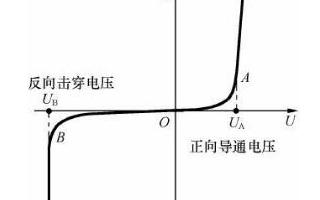
The figure shows the volt ampere characteristic curve of the diode. It can be seen from the figure that the current in the reverse cut-off area is not completely 0, and our COMS is actually made of PN structure, so it conforms to this characteristic, and the photodiode works under the reverse voltage, so the small current without light is dark current.
Add a fixed value before AD
-
There will be an ad conversion process from sensor to ISP, and the ad chip will have a sensitivity. When the voltage is lower than this threshold, AD conversion cannot be carried out, so a constant is artificially added so that the value originally lower than the threshold can also be ad converted;
-
Because the human eye is more sensitive to dark details and less sensitive to highlights, a constant is added to preserve larger dark details at the expense of light areas that are not sensitive to the human eye.

The above two points mean to raise AB to A'B ', so that the values in this interval can complete AD conversion, and this area can better retain the dark area, that is, the sensitive part of the human eye, at the expense of the BC part, because this part of the information is insensitive to the human eye, which is more in line with the needs of the human eye.
BL correction
BL correction is generally divided into sensor side and ISP side, but our column focuses on the algorithm in ISP PIPELINE, so the algorithm in sensor is not discussed.
SENSOR end
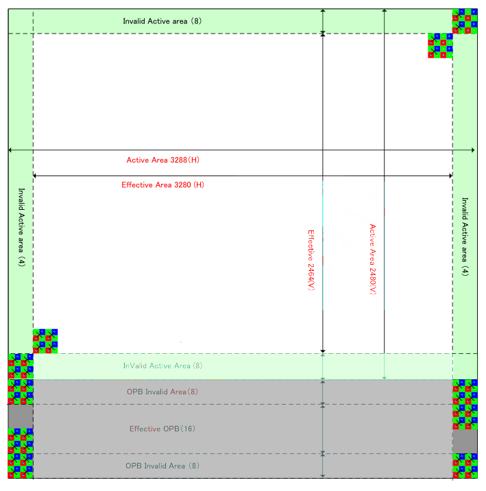
As shown in the figure, this is the distribution of a sensor pixel array. The maximum mapping resolution of this sensor is 3280 * 2464, which is the effective pixel area. Then there is an effective OPB area in the gray part below, which is the sensor ob area. The biggest difference between the two parts is that the effective pixel area can be exposed normally, while the OB area cannot accept photons in technology. The simplest idea is to coat a layer of black non photosensitive material on the photosensitive display, so that the value of effective pixels can be corrected by the value of no light in the OB area. The simplest operation is to average the pixel values of ob, and then subtract this value from each pixel value to complete the correction. Of course, now the sensor will also have some high-end correction algorithms.
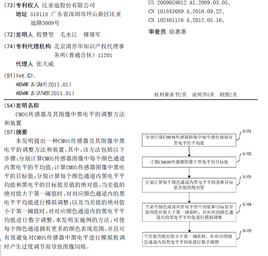
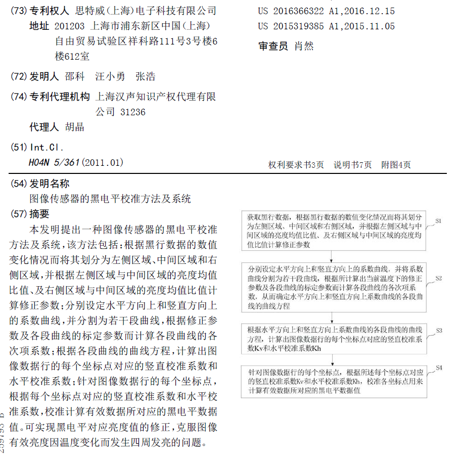
As shown in the figure, Stevie and BYD proposed two more advanced algorithms. As just said, the processing of sensor is not the focus of this column, so there is no key explanation. Those who are interested can study by themselves, and those who need information can leave a message.
ISP end
The algorithms at the ISP end all pass through a black frame RAW graph, and then operate the RAW graph. The following is an 8-bit description.
Deducting fixed value method
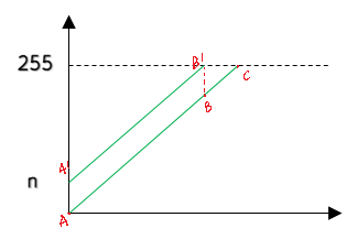
The method of deducting fixed value is to deduct A fixed value from each channel, as shown in the figure above, just translate A'b 'to AB.
The specific methods are as follows:
-
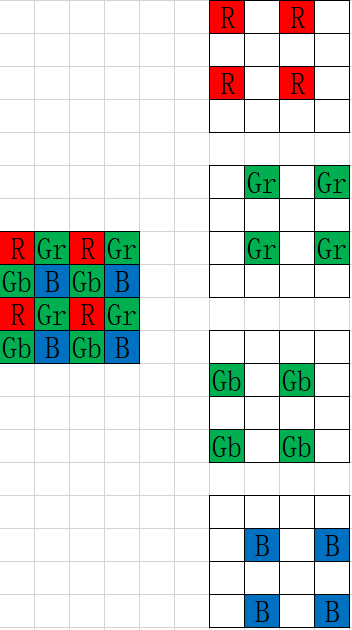
Collect the black frame RAW diagram and divide it into four channels: GR, GB, R and B;
-
Average the four channels (some algorithms also use median value or other methods);
-
Each channel of the subsequent image subtracts the correction value of each channel calculated in 2;
-
Normalize Gr and Gb channels, that is, after A'B 'is translated to AB, the maximum value is the ordinate of point B, but we need to restore this value to 255 so that the restored pixel value range is still 0-255;
Gin × 255 255 − B L \operatorname{Gin} \times \frac{255}{255-B L} Gin×255−BL255
The correction can be completed through the above formula. It should be noted that the RB channel does not need to be normalized to the 0-255 range, because its range will be increased to 0-255 through gain in the subsequent AWB, which will be discussed later in the AWB algorithm.
At present, this method is often used. For example, Hisilicon and Sonix I contacted use this simple and rough method. As mentioned above, the Sensor end will have a BL processing, so the back end can also complete the correction through this simple method.
ISO linkage method
Because the dark current is related to gain value and temperature, the correction value under each condition is determined by linkage. Then, check the corresponding correction value through the parameters for correction.
The specific methods are as follows:
- Initialize an ISO value (in fact, the combination of AG and DG), then repeat the practice in the fixed value, collect black frames and calibrate the correction values of each channel;
- On the basis of initializing ISO, increase ISO by means of equal difference or equal ratio sequence, and then repeat step 1 to obtain the correction value of each channel;
- The two-dimensional data is made into a LUT, and the subsequent images are corrected by finding the corresponding correction value through the ISO value. The parameters of ISO value not in LUT can be obtained by interpolation.
Curve fitting method
The correction value of each channel corrected by the above two methods is a fixed value, but we know that the actual data of black frames at different positions of pixels are different, so a more accurate way is to calculate a correction value for each point to correct the point. But now the general pixel values are very high, so it is impossible to save the values of each point, so the memory demand is too large, so it is the same as oversampling. It is to select some pixels in the black frame to calculate the correction value of the point, and then store the coordinates and correction values in a LUT. The correction values of other subsequent pixels can be obtained through the progressive interpolation of coordinates and this LUT, so as to realize the accurate correction of each point.
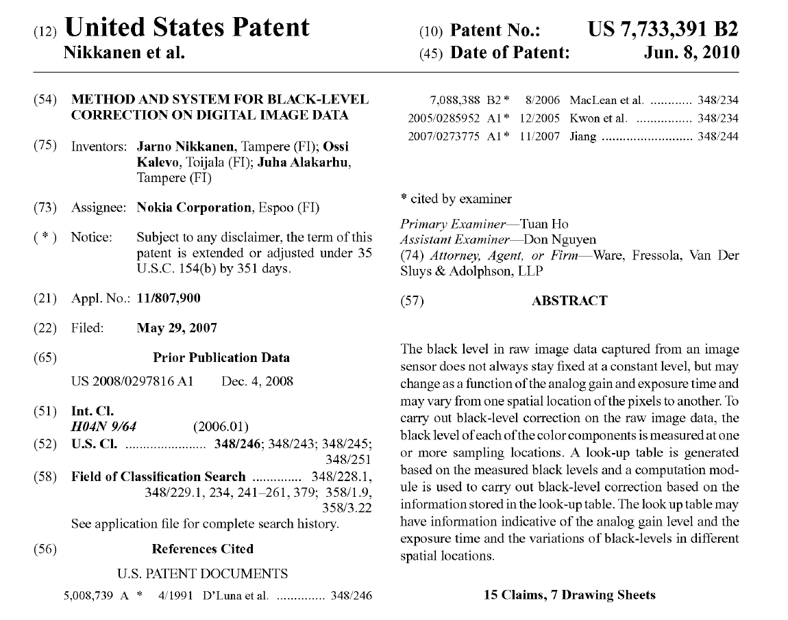
As shown in the figure, the patent establishes the LUT of AG, the LUT of exposure time, and then the LUT of coordinates, which is equivalent to adding coordinate position information on the basis of ISO linkage mode to realize the accurate correction of each point.
Correction summary
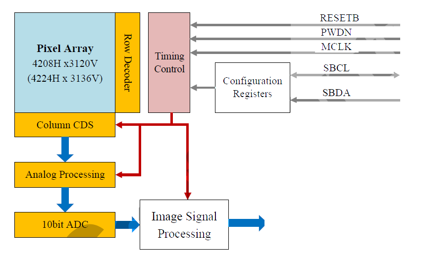
The figure is a data flow chart. It can be seen that the sensor end can carry out analog processing and digital processing, while the ISP end can carry out digital processing intelligently. Because the signal received by the ISP is a digital signal after AD conversion, the processing at the sensor end can be more refined. As mentioned in the above bidi patent, the thick bar at the sensor end can be processed through analog signal, Then fine tune, and then deal with it through digital processing. Therefore, to sum up, generally, the ISP can be completed through relatively simple correction, which can save hardware resources. This is the reason why most of the processing methods used by ISP chips are very simple.
Concrete implementation
%% --------------------------------
%% author:wtzhu
%% date: 20210629
%% fuction: main file of BLC
%% --------------------------------
clc;clear;close all;

% ------------Raw Format----------------
filePath = 'images/HisiRAW_4208x3120_8bits_RGGB.raw';
bayerFormat = 'RGGB';
row = 4208;
col = 3120;
bits = 8;
% --------------------------------------

%  I(1:2:end, 1:2:end) = R(1:1:end, 1:1:end);

data = readRaw(filePath, bits, row, col);
% get the four channels by bayerFormat
switch bayerFormat
    case 'RGGB'
        disp('bayerFormat: RGGB');
        R = data(1:2:end, 1:2:end);
        Gr = data(1:2:end, 2:2:end);
        Gb = data(2:2:end, 1:2:end);
        B = data(2:2:end, 2:2:end);
    case 'GRBG'
        disp('bayerFormat: GRBG');
        Gr = data(1:2:end, 1:2:end);
        R = data(1:2:end, 2:2:end);
        B = data(2:2:end, 1:2:end);
        Gb = data(2:2:end, 2:2:end);
    case 'GBRG'
        disp('bayerFormat: GBRG');
        Gb = data(1:2:end, 1:2:end);
        B = data(1:2:end, 2:2:end);
        R = data(2:2:end, 1:2:end);
        Gr = data(2:2:end, 2:2:end);
    case 'BGGR'
        disp('bayerFormat: BGGR');
        B = data(1:2:end, 1:2:end);
        Gb = data(1:2:end, 2:2:end);
        Gr = data(2:2:end, 1:2:end);
        R = data(2:2:end, 2:2:end);
end
% calculate the Correction coefficient of every channel
R_mean = round(mean(mean(R)));
Gr_mean = round(mean(mean(Gr)));
Gb_mean = round(mean(mean(Gb)));
B_mean = round(mean(mean(B)));

% Correct each channel separately
cR = R-R_mean;
cGr = Gr-Gr_mean;
cGb = Gb-Gb_mean;
cB = B-B_mean;
fprintf('R:%d Gr:%d Gb:%d B:%d\n', R_mean, Gr_mean, Gb_mean, B_mean);

cData = zeros(size(data));
% Restore the image with four channels
switch bayerFormat
    case 'RGGB'
        disp('bayerFormat: RGGB');
        cData(1:2:end, 1:2:end) = cR(1:1:end, 1:1:end);
        cData(1:2:end, 2:2:end) = cGr(1:1:end, 1:1:end);
        cData(2:2:end, 1:2:end) = cGb(1:1:end, 1:1:end);
        cData(2:2:end, 2:2:end) = cB(1:1:end, 1:1:end);
    case 'GRBG'
        disp('bayerFormat: GRBG');
        cData(1:2:end, 1:2:end) = cGr(1:1:end, 1:1:end);
        datacData(1:2:end, 2:2:end) = cR(1:1:end, 1:1:end);
        cData(2:2:end, 1:2:end) = cB(1:1:end, 1:1:end);
        data(2:2:end, 2:2:end) = cGb(1:1:end, 1:1:end);
    case 'GBRG'
        disp('bayerFormat: GBRG');
        cData(1:2:end, 1:2:end) = cGb(1:1:end, 1:1:end);
        cData(1:2:end, 2:2:end) = cB(1:1:end, 1:1:end);
        cData(2:2:end, 1:2:end) = cR(1:1:end, 1:1:end);
        cData(2:2:end, 2:2:end) = cGr(1:1:end, 1:1:end);
    case 'BGGR'
        disp('bayerFormat: BGGR');
        cData(1:2:end, 1:2:end) = cB(1:1:end, 1:1:end);
        cData(1:2:end, 2:2:end) = cGb(1:1:end, 1:1:end);
        cData(2:2:end, 1:2:end) = cGr(1:1:end, 1:1:end);
        cData(2:2:end, 2:2:end) = cR(1:1:end, 1:1:end);
end
show(data, cData, bits, Gr_mean);
readRaw.m:
function rawData = readRaw(fileName, bitsNum, row, col)
% readRaw.m    get rawData from HiRawImage
%   Input:
%       fileName    the path of HiRawImage
%       bitsNum      the number of bits of raw image
%       row         the row of the raw image
%       col         the column of the raw image
%   Output:
%       rawData     the matrix of raw image data
%   Instructions:
%       author:     wtzhu
%       e-mail:     wtzhu_13@163.com
% Last Modified by wtzhu v1.0 2021-06-29
% Note:

% get fileID
fin = fopen(fileName, 'r');
% format precision
switch bitsNum
    case 8
        disp('bits: 8');
        format = sprintf('uint8=>uint8');
    case 10
        disp('bits: 10');
        format = sprintf('uint16=>uint16');
    case 12
        disp('bits: 12');
        format = sprintf('uint16=>uint16');
    case 16
        disp('bits: 16');
        format = sprintf('uint16=>uint16');
end
I = fread(fin, row*col, format);
% plot(I, '.');
z = reshape(I, row, col);
z = z';
rawData = z;
% imshow(z);
end
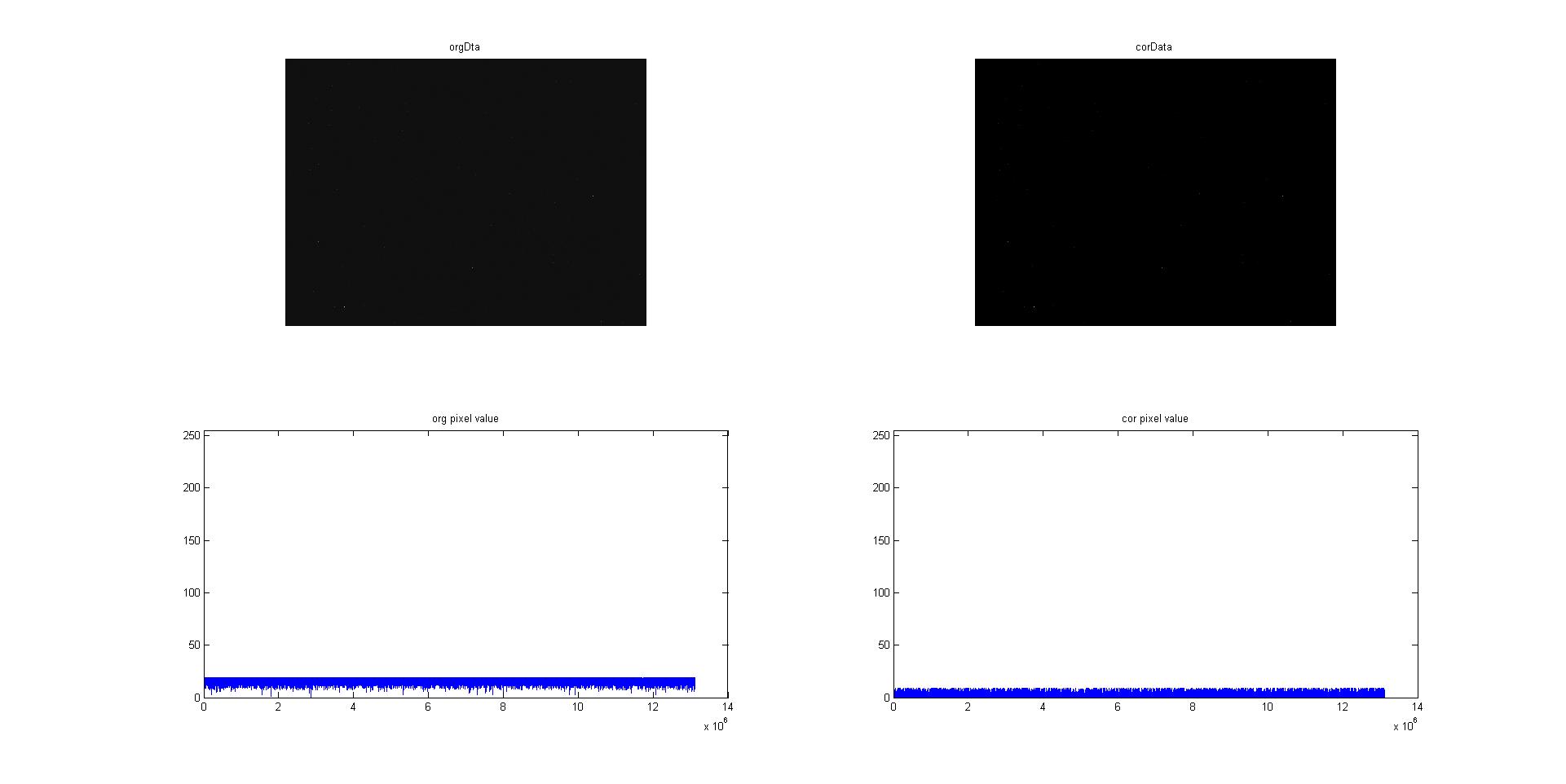
Correction effect
Tips:
- In order to facilitate downloading, this project has not been updated to github. gitee can be used in ISPAlgorithmStudy: ISP algorithm learning summary, mainly paper summary (gitee.com) Obtain relevant data codes from the warehouse.
- In this phase, station B has video synchronization explanation, ISP algorithm elaboration - BLC_ Beep beep beep_ bilibili , you can pay attention to station B, and there will be more video explanation and synchronization of algorithms in the future;
- Zhihu column ISP image processing - Zhihu (zhihu.com) There will also be algorithm synchronization;