This part does not pay attention to the derivation of Kalman filter, but only the function of Kalman filter [it is said that the derivation is difficult 😒😒， In short, this article is to explain the overall process of Kalman filter without the step-by-step derivation of tangled formula. After reading this part, you will know what Kalman filter does and what the specific steps are ✔✔]

What does Kalman filter do

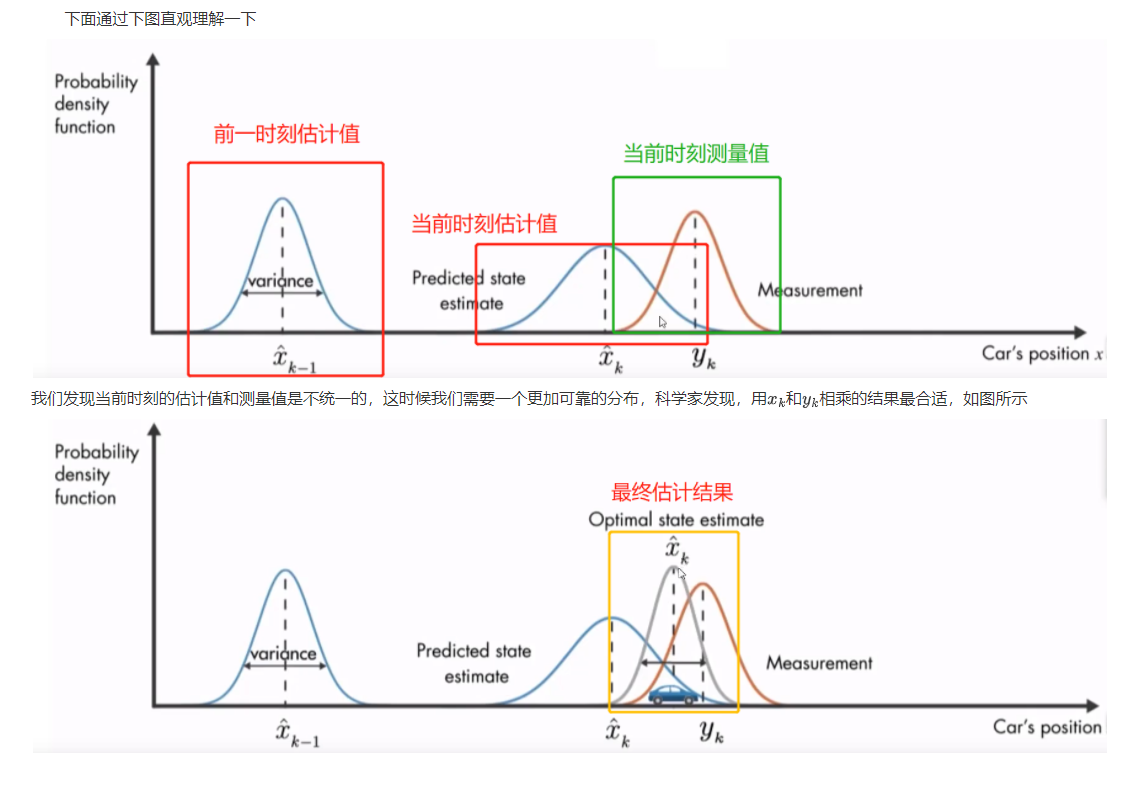
Kalman filter is used to estimate the state of things. Why estimate the state of things? It must be that we can't accurately know the current state of things, At this time, we have to make an estimate [however, we can't estimate casually. We often estimate based on some experience, and the results of all estimates are relatively accurate]; on the other hand, in order to estimate the state of a thing, we can also use some instruments to measure, but there will be some measurement error when measuring with instruments. At this time, a problem will arise, and we should Should we trust our estimates or measurements? I think most people think so: if the measuring instruments we use are inferior instruments bought for 50 cents from a small manufacturer, we will trust the estimation results more; If the instrument is worth thousands of gold, we have reason to believe the measurement results. In fact, we often assign different proportions to these two results, indicating which result we trust more. Then Kalman filter is a method to estimate the state of things by combining the prior estimation and instrument measurement.

Let's give another example to illustrate the meaning of the above. As shown in the figure below, we use the stove to boil water for the kettle. Now the water is boiling. Combined with the knowledge of junior middle school, we estimate that the water temperature is 95.4 ° C [affected by atmospheric pressure, not 100 degrees] 🎈]， That is, Xk=95.4 ° C. At this time, we use a thermometer to measure the temperature of water and find that its value is yk=94.1 ° C. If you find that xk and yk are inconsistent, who should you trust? Assuming that the reliability of the thermometer is 0.6 and the estimated value is 0.4, the final water temperature = 0.6 * 94.1 + 0.4 * 95.4 = 94.62.

Example analysis of Kalman filter

Kalman formula

Kalman is mainly the five formulas in the figure above. First, predict the state of the object, and then update the measurement, so as to cycle.

Intuitive understanding of Kalman filter

​

Kalman Python example [using Jupiter notebook]

This example mainly produces some position and speed information randomly, and then estimates the traveler's speed and position through Kalman filter.

#Load related libraries
import numpy as np
%matplotlib inline
import matplotlib.pyplot as plt
from scipy.stats import norm

#Initialize pedestrian state x, pedestrian uncertainty (covariance matrix) P, measured time interval dt, processing matrix F and measurement matrix H:
x = np.matrix([[0.0, 0.0, 0.0, 0.0]]).T
print(x, x.shape)
P = np.diag([1000.0, 1000.0, 1000.0, 1000.0])
print(P, P.shape)

dt = 0.1 # Time Step between Filter Steps
F = np.matrix([[1.0, 0.0, dt, 0.0],
              [0.0, 1.0, 0.0, dt],
              [0.0, 0.0, 1.0, 0.0],
              [0.0, 0.0, 0.0, 1.0]])
print(F, F.shape)

H = np.matrix([[0.0, 0.0, 1.0, 0.0],
              [0.0, 0.0, 0.0, 1.0]])
print(H, H.shape)

ra = 10.0**2

R = np.matrix([[ra, 0.0],
              [0.0, ra]])
print(R, R.shape)

#The covariance matrix R of the noise in the measurement process and the covariance matrix Q of the process noise are calculated
ra = 0.09
R = np.matrix([[ra, 0.0],
              [0.0, ra]])
print(R, R.shape)

sv = 0.5
G = np.matrix([[0.5*dt**2],
               [0.5*dt**2],
               [dt],
               [dt]])
Q = G*G.T*sv**2
from sympy import Symbol, Matrix
from sympy.interactive import printing
printing.init_printing()
dts = Symbol('dt')
Qs = Matrix([[0.5*dts**2],[0.5*dts**2],[dts],[dts]])
Qs*Qs.T

I = np.eye(4)
print(I, I.shape)

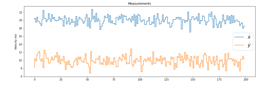
#Randomly generate some measurement data
m = 200 # Measurements
vx= 20 # in X
vy= 10 # in Y

mx = np.array(vx+np.random.randn(m))
my = np.array(vy+np.random.randn(m))
measurements = np.vstack((mx,my))

print(measurements.shape)
print('Standard Deviation of Acceleration Measurements=%.2f' % np.std(mx))
print('You assumed %.2f in R.' % R[0,0])

fig = plt.figure(figsize=(16,5))
plt.step(range(m),mx, label='$\dot x$')
plt.step(range(m),my, label='$\dot y$')
plt.ylabel(r'Velocity $m/s$')
plt.title('Measurements')
plt.legend(loc='best',prop={'size':18})

#Some process values are used for the display of results
xt = []
yt = []
dxt= []
dyt= []
Zx = []
Zy = []
Px = []
Py = []
Pdx= []
Pdy= []
Rdx= []
Rdy= []
Kx = []
Ky = []
Kdx= []
Kdy= []

def savestates(x, Z, P, R, K):
    xt.append(float(x[0]))
    yt.append(float(x[1]))
    dxt.append(float(x[2]))
    dyt.append(float(x[3]))
    Zx.append(float(Z[0]))
    Zy.append(float(Z[1]))
    Px.append(float(P[0,0]))
    Py.append(float(P[1,1]))
    Pdx.append(float(P[2,2]))
    Pdy.append(float(P[3,3]))
    Rdx.append(float(R[0,0]))
    Rdy.append(float(R[1,1]))
    Kx.append(float(K[0,0]))
    Ky.append(float(K[1,0]))
    Kdx.append(float(K[2,0]))
    Kdy.append(float(K[3,0]))    

#Kalman filtering 
for n in range(len(measurements[0])):
 
    # Time Update (Prediction)
    # ========================
    # Project the state ahead
    x = F*x
    
    # Project the error covariance ahead
    P = F*P*F.T + Q
    
    # Measurement Update (Correction)
    # ===============================
    # Compute the Kalman Gain
    S = H*P*H.T + R
    K = (P*H.T) * np.linalg.pinv(S)
    
    # Update the estimate via z
    Z = measurements[:,n].reshape(2,1)
    y = Z - (H*x)                            # Innovation or Residual
    x = x + (K*y)
    
    # Update the error covariance
    P = (I - (K*H))*P
    
    # Save states (for Plotting)
    savestates(x, Z, P, R, K)

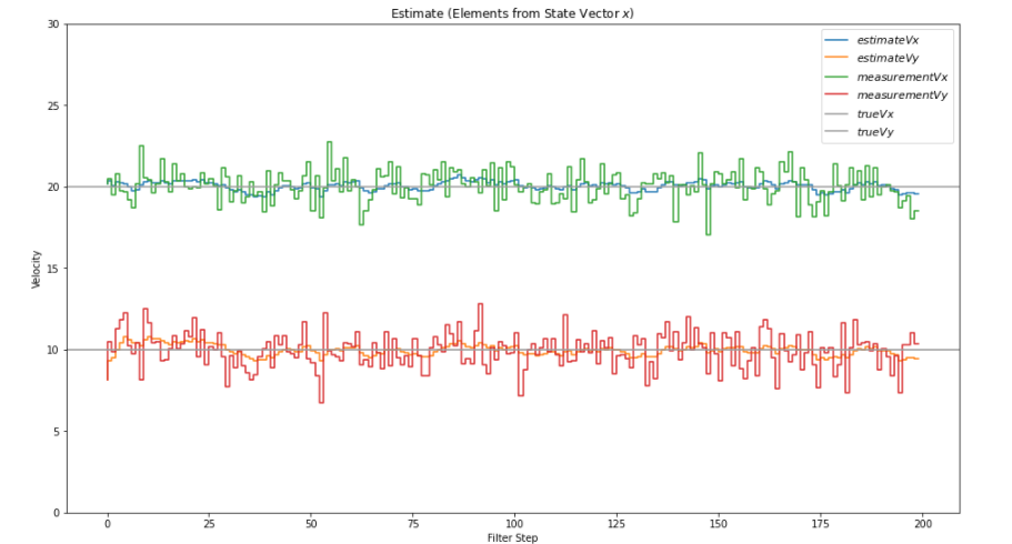
#Show me the estimated speed
def plot_x():
    fig = plt.figure(figsize=(16,9))
    plt.step(range(len(measurements[0])),dxt, label='$estimateVx$')
    plt.step(range(len(measurements[0])),dyt, label='$estimateVy$')
    
    plt.step(range(len(measurements[0])),measurements[0], label='$measurementVx$')
    plt.step(range(len(measurements[0])),measurements[1], label='$measurementVy$')

    plt.axhline(vx, color='#999999', label='$trueVx$')
    plt.axhline(vy, color='#999999', label='$trueVy$')

    plt.xlabel('Filter Step')
    plt.title('Estimate (Elements from State Vector $x$)')
    plt.legend(loc='best',prop={'size':11})
    plt.ylim([0, 30])
    plt.ylabel('Velocity')
plot_x()

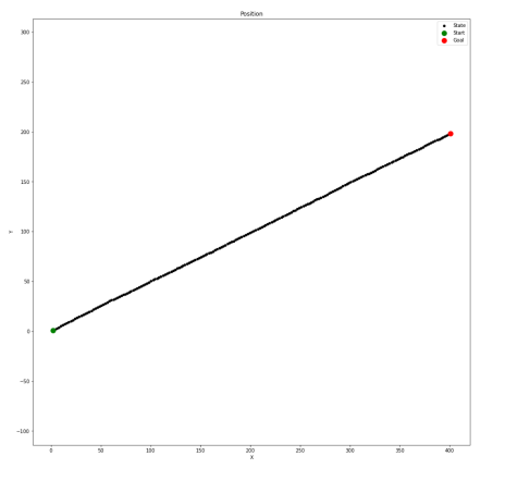
#Displays the estimated results of the location
def plot_xy():
    fig = plt.figure(figsize=(16,16))
    plt.scatter(xt,yt, s=20, label='State', c='k')
    plt.scatter(xt[0],yt[0], s=100, label='Start', c='g')
    plt.scatter(xt[-1],yt[-1], s=100, label='Goal', c='r')

    plt.xlabel('X')
    plt.ylabel('Y')
    plt.title('Position')
    plt.legend(loc='best')
    plt.axis('equal')
plot_xy()