Recently, in order to complete the license plate recognition, I'm going to learn opencv. Here, I'll record the learning process and notes
Image manipulation
imread read image
Use cv The imread() function reads the image. The image should be in the working directory or the full path of the image should be given.
The second parameter is a flag that specifies how the image is read.
cv.IMREAD_COLOR: load color image. The transparency of any image is ignored. It is the default flag.
cv.IMREAD_GRAYSCALE: loads images in grayscale mode
cv.IMREAD_UNCHANGED: loads images, including alpha channels
Note that in addition to these three flags, you can simply pass integers 1, 0, or - 1, respectively.
cv2.imread() saves the picture information in the form of multi-dimensional array after reading the picture. The first two dimensions represent the pixel coordinates of the picture, and the last one dimension represents the channel index of the picture. The number of channels of the specific image is determined by the format of the picture
if __name__ == '__main__':
    car=cv2.imread('./car4.jpg')
    print(car.shape) #(300, 560, 3) array shape height: 300 pixels width: 560 pixels 3D
    print(type(car)) #numpy array
    print(car) #3D array (color image: height, width, pixels, red, green and blue)
    cv2.imshow('car',car[::-1,:,:]) # Pop up window
    #The first dimension represents height:: - 1 represents flip, upside down, upside down
    #The second dimension represents the width
    #The third dimension represents the color blue 0 green 1 red 2
    cv2.waitKey() #Wait for keyboard input and arbitrary output, send this code, and the window disappears. 0 means infinite waiting; 1000 ms
    cv2.destroyAllWindows() #Destroy memory
import cv2
import numpy as np
if __name__ == '__main__':
img = cv2.imread('car4.jpg', cv2.IMREAD_UNCHANGED) # Contains alpha channels
cv2.imshow('car',img)
img2 = cv2.imread('car4.jpg', cv2.IMREAD_COLOR) # color image
cv2.imshow('car2',img2)
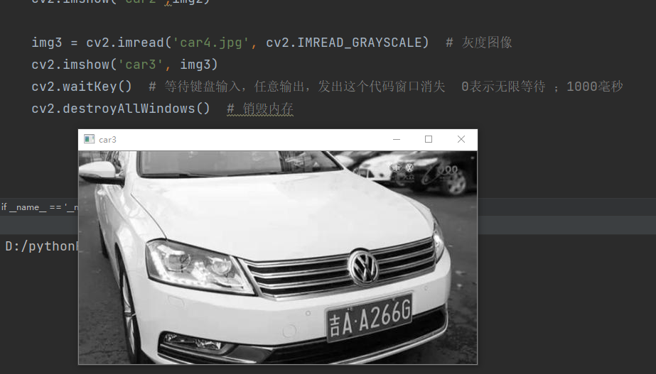
img3 = cv2.imread('car4.jpg', cv2.IMREAD_GRAYSCALE) # Gray image
cv2.imshow('car3', img3)
cv2.waitKey() # Wait for keyboard input and arbitrary output, send this code, and the window disappears. 0 means infinite waiting; 1000 ms
cv2.destroyAllWindows() # Destroy memory
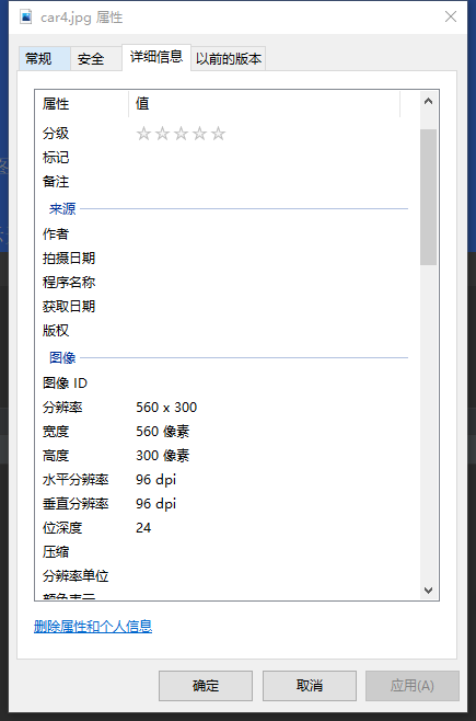
As you can see from the details, car4 Jpg contains three channels (R G B), that is, the bit depth is 24, and each channel occupies 8 bits, so it does not contain alpha channel, so the first two read out the same effect
imshow display image
Use function * * cv Imshow() * * displays the image in the window. The window automatically fits the image size.
The first parameter is the window name, which is a string. The second parameter is our object. You can create as many windows as you want, but you can use different window names.
img3 = cv2.imread('car4.jpg', cv2.IMREAD_GRAYSCALE)  # Gray image
    cv2.imshow('car3', img3)
    cv2.waitKey()  # Wait for keyboard input and arbitrary output, send this code, and the window disappears. 0 means infinite waiting; 1000 ms
    cv2.destroyAllWindows()  # Destroy memory
waitKey
waitKey() is a keyboard binding function. The parameter is the time in milliseconds. This function waits for the specified milliseconds for any keyboard event. If you press any key during this time, the program will continue to run. If 0 is passed, it will wait indefinitely for a keystroke. It can also be set to detect specific keys, for example, if key a is pressed, we will discuss it below.
Note that in addition to keyboard binding events, this feature handles many other GUI events, so you must use it to actually display images.
cv.destroyAllWindows() will only destroy all the windows we created. If you want to destroy any particular window, use the function cv Destroywindow() passes the exact window name as a parameter.
Note that in special cases, you can create an empty window and then load the image into the window. In this case, you can specify whether the window can be resized. This is through the function cv Namedwindow() completed. By default, this flag is cv WINDOW_ AUTOSIZE. However, if the flag is specified as CV WINDOW_ Normal, you can resize the window. This is helpful when the image size is too large and when adding a tracking bar to the window.
cv.namedWindow('image',cv.WINDOW_NORMAL)
cv.imshow('image',img)
cv.waitKey(0)
cv.destroyAllWindows()
resize changes the size of the image
Function function: reduce or enlarge the function to a certain size
resize(InputArray src, OutputArray dst, Size dsize,
        double fx=0, double fy=0, int interpolation=INTER_LINEAR )
Parameter interpretation:
InputArray src: input the original image, that is, the image to be changed in size;
OutputArray dst: output the changed image. This image has the same content as the original image, but the size is different from the original image;
dsize: the size of the output image.
If this parameter is not 0, it means that the original image is scaled to the size specified by the Size(width, height); If this parameter is 0, the size of the original image after scaling shall be calculated by the following formula:
dsize = Size(round(fxsrc.cols), round(fysrc.rows))
Among them, fx and fy are the two parameters to be mentioned below, which are the scaling scale in the width direction and height direction of the image.
fx: the scale in the width direction. If it is 0, it will follow (double) dsize width/src. Cols;
fy: the scaling scale in the height direction. If it is 0, it will follow (double) dsize height/src. Rows to calculate;
Precautions for use:
dsize and fx/fy cannot be 0 at the same time,
Or you can specify the value of dsize and let fx and fy empty and directly use the default value, such as resize(img, imgDst, Size(30,30));
Or you can set dsize to 0 and specify the values of fx and fy, such as fx=fy=0.5, which is equivalent to doubling the two directions of the original image!
img.shape #(300, 560, 3) array shape height: 300 pixels width: 560 pixels 3D height first and then width
resize is the first width in height
	car=cv2.imread('./car4.jpg')
    car2=cv2.resize(car,(150,280))
    cv2.imshow('car',car) # Pop up window
    cv2.waitKey() #Wait for keyboard input and arbitrary output, send this code, and the window disappears. 0 means infinite waiting; 1000 ms
    cv2.destroyAllWindows() #Destroy memory
cvtColor change color
cvtcolor() function is a color space conversion function, which can convert RGB color to HSV, HSI and other color spaces. It can also be converted to grayscale image
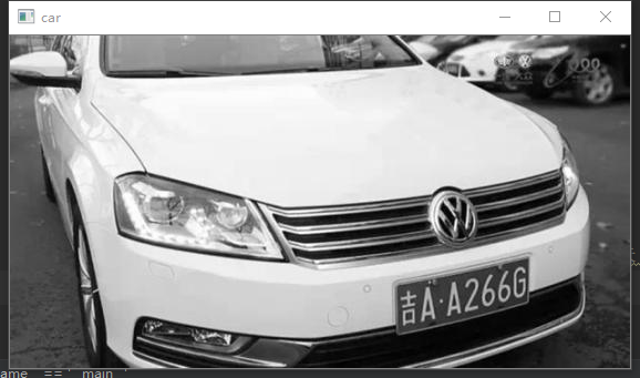
   car=cv2.imread('./car4.jpg')

    car2=cv2.cvtColor(car,code=cv2.COLOR_BGR2GRAY)
    cv2.imshow('car',car2) # Pop up window
    cv2.waitKey() #Wait for keyboard input and arbitrary output, send this code, and the window disappears. 0 means infinite waiting; 1000 ms
    cv2.destroyAllWindows() #Destroy memory
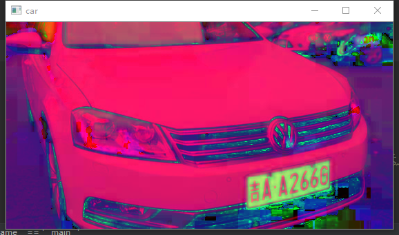
 car=cv2.imread('./car4.jpg')

    car2=cv2.cvtColor(car,code=cv2.COLOR_BGR2HSV)
    cv2.imshow('car',car2) # Pop up window
    cv2.waitKey() #Wait for keyboard input and arbitrary output, send this code, and the window disappears. 0 means infinite waiting; 1000 ms
    cv2.destroyAllWindows() #Destroy memory
imwrite write image
Use the function cv Imwrite() saves the image.
The first parameter is the file name, and the second parameter is the image to be saved. cv.imwrite(‘messigray.png’,img)
This saves the image in PNG format in the working directory.
img3 = cv2.imread('car4.jpg', cv2.IMREAD_GRAYSCALE)  # Gray image
cv2.imwrite('./car3.jpg',img3)
hsv
HSV(Hue, Saturation, Value) is a color space based on the intuitive characteristics of color
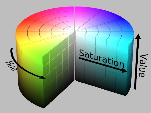
The color parameters in this model are hue (H), saturation (S) and lightness (V)
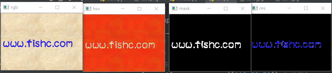
import cv2
import numpy as np
if __name__ == '__main__':
    img1 = cv2.imread('./test.png') # Color space BGR
    img2 = cv2.cvtColor(img1,code = cv2.COLOR_BGR2HSV) # Transformation of color space
    # Defines the range of blue in the HSV color space
    lower_blue = np.array([110,50,50]) # wathet
    upper_blue = np.array([130,255,255]) # navy blue
    # Mark which positions in the picture are blue according to the range of blue
    # Is inRange within this range lower_bule ~ upper_blue: Blue
    # If it is, it is 255, otherwise it is 0
    mask = cv2.inRange(img2,lower_blue,upper_blue)
    res = cv2.bitwise_and(img1, img1,mask = mask) # Bit operation: and operation!
    cv2.imshow('rgb',img1)
    cv2.imshow('hsv',img2)
    cv2.imshow('mask',mask)
    cv2.imshow('res',res)

    cv2.waitKey(0)
    cv2.destroyAllWindows() # Keyboard input, window, destroy, free memory
How do I find the HSV value to track?
This is in stackoverflow Com. It's very simple. You can use the same function cv cvtColor(). You just need to pass the BGR value you want, not the image. For example, to find a green HSV value,
green = np.uint8([[[0,255,0 ]]])
hsv_green = cv.cvtColor(green,cv.COLOR_BGR2HSV)
print( hsv_green )

[[[ 60 255 255]]]
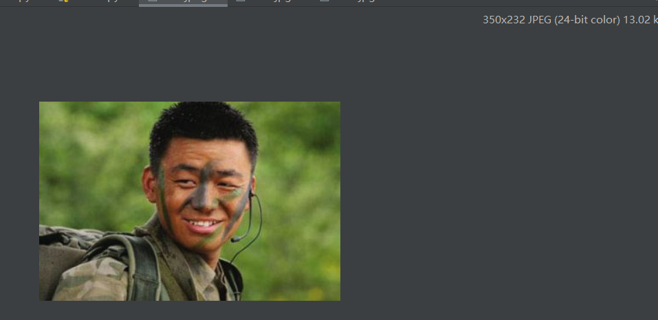
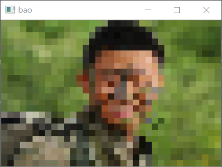
Mosaic
Later, we will take this picture as an example, 350 wide and 232 high
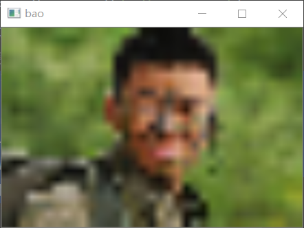
Mosaic mode I
It is to shrink the picture first and enlarge it. In fact, it is to blur the picture
import cv2
import numpy as np

if __name__ == '__main__':
    img = cv2.imread('./bao.jpeg')
    print(img.shape) # Height 232, width 350
    # Mosaic mode I
    img2 = cv2.resize(img,(35,23))
    img3 = cv2.resize(img2,(350,232))
    cv2.imshow('bao',img3)
    cv2.waitKey(0)
    cv2.destroyAllWindows()
Mosaic mode II
import cv2
import numpy as np

if __name__ == '__main__':
    img = cv2.imread('./bao.jpeg')
    print(img.shape)  # Height 232, width 350
    img2 = cv2.resize(img,(35,23))  #Shrink 10 times first
    img3 = np.repeat(img2,10,axis=0) # Repeat line
    img4 = np.repeat(img3,10,axis=1) # Duplicate column
    cv2.imshow('bao',img4)
    cv2.waitKey(0)
    cv2.destroyAllWindows()

Mosaic mode III
import cv2
import numpy as np

if __name__ == '__main__':
    img = cv2.imread('./bao.jpeg')
    print(img.shape)  # Height 232, width 350
    # Mosaic mode 3
    img2 = img[::10, ::10]  # One pixel out of every 10, details
    cv2.namedWindow('bao', flags=cv2.WINDOW_NORMAL)
    cv2.resizeWindow('bao', 350, 232)
    cv2.imshow('bao', img2)
    cv2.waitKey(0)
    cv2.destroyAllWindows()
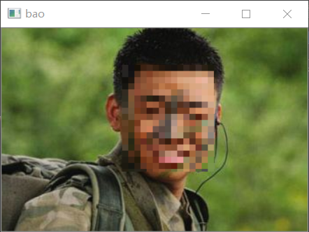
Face mosaic
import numpy as np
import cv2
if __name__ == '__main__':
    img = cv2.imread('./bao.jpeg')
    # 1. Human face location
    # Coordinates of the upper left corner of the face (143, 42); Lower right corner (239164) (x,y) (width, height)
    # 2. Slice to get face
    face = img[42:164,138:244]
    # 3. Interval slice, repeat, slice, assignment
    face = face[::7,::7] # One pixel out of every seven, mosaic
    face = np.repeat(face,7,axis = 0) # Repeat 7 times in the row direction
    face = np.repeat(face, 7, axis=1) # Repeat 7 times in the column direction
    img[42:164,138:244] = face[:122,:106] # Filling, uniform size
    # 4. Show
    cv2.imshow('bao',img)
    cv2.waitKey(0)
    cv2.destroyAllWindows()
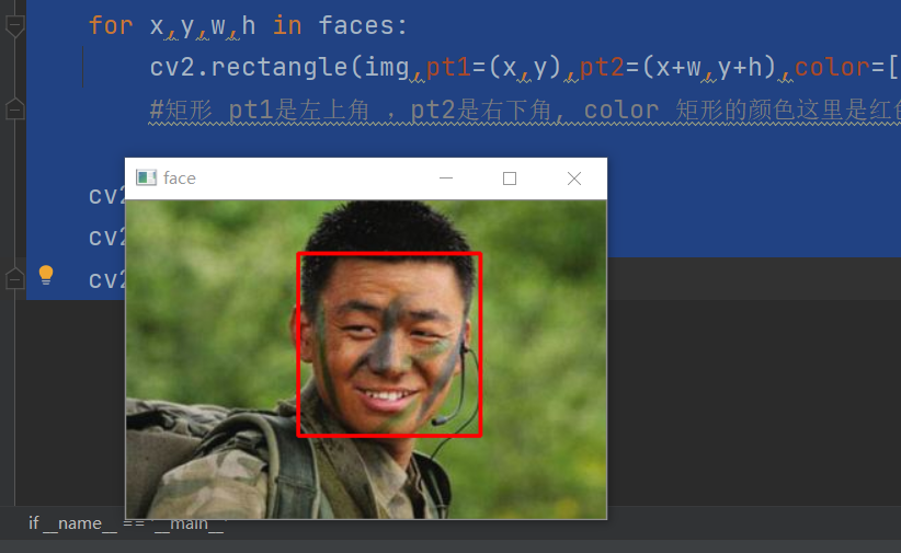
Face detection
First, go to github and search opencv,
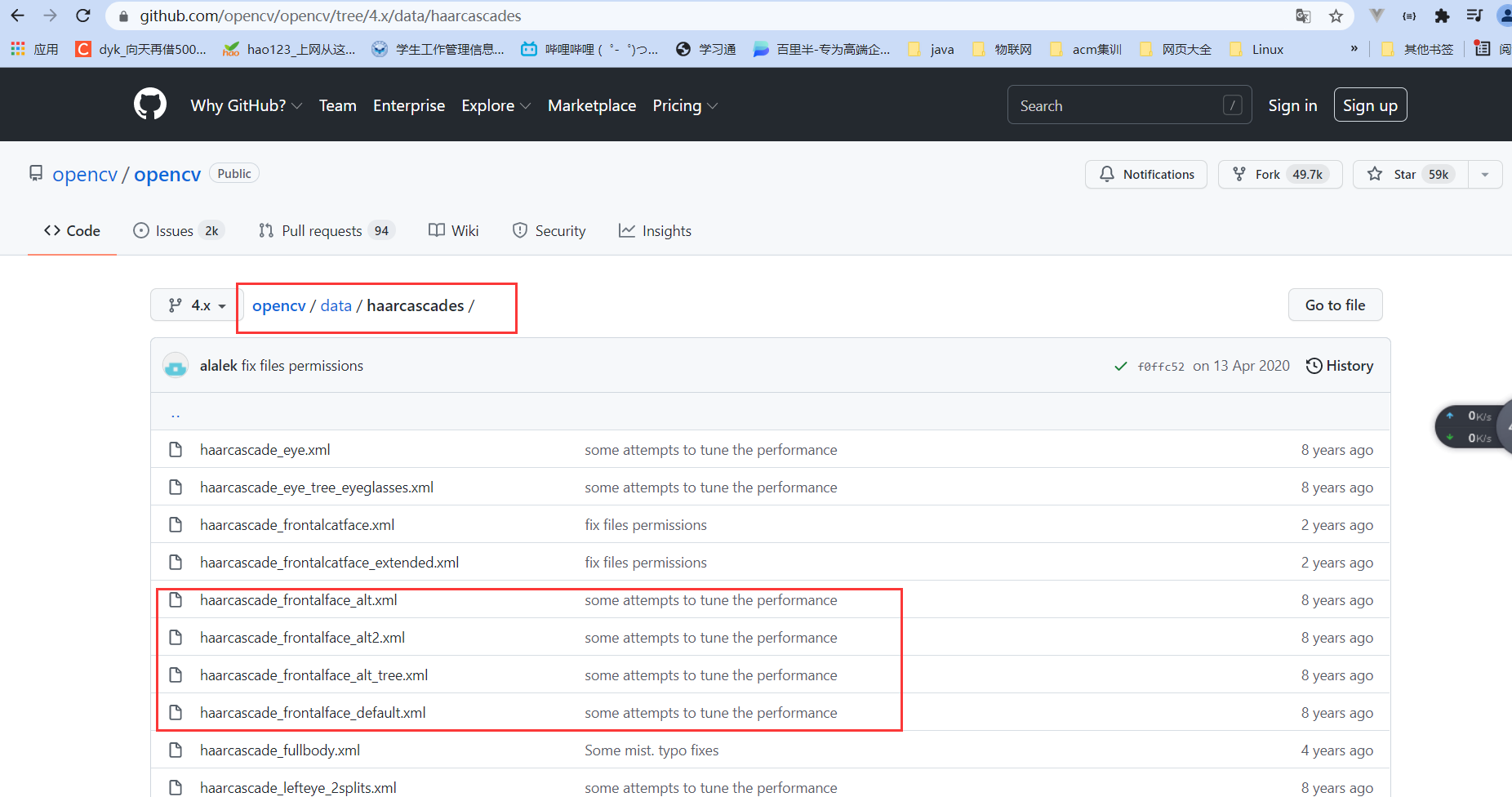
The first feature I use here is xml
import numpy as np
import cv2

if __name__ == '__main__':
    img = cv2.imread('./bao.jpeg')

    # Detailed description of face features, more than 10000 lines. The computer carries out face detection according to these features
    # According to one part, it is regarded as a face
    # Cascade classifier, detector,
    face_detector = cv2.CascadeClassifier('./haarcascade_frontalface_alt.xml')
    faces=face_detector.detectMultiScale(img) # The first two are face coordinates x, y, and the last two are width and height

    print(faces) # [[125  38 133 133]] x,y,w,h
    for x,y,w,h in faces:
        cv2.rectangle(img,pt1=(x,y),pt2=(x+w,y+h),color=[0,0,255],thickness=2)
        #Rectangle pt1 is the upper left corner, pt2 is the lower right corner, and the color of color rectangle is red here. The greater the thickness value, the thicker it is

    cv2.imshow('face',img)
    cv2.waitKey(0)
    cv2.destroyAllWindows()
Multiple face detection
import numpy as np
import cv2

if __name__ == '__main__':
    img = cv2.imread('./sew2.jpeg')
    gray = cv2.cvtColor(img,code=cv2.COLOR_BGR2GRAY) # Using gray can reduce data
    # Detailed description of face features, more than 10000 lines. The computer carries out face detection according to these features
    # According to one part, it is regarded as a face
    # Cascade classifier, detector,
    face_detector = cv2.CascadeClassifier('./haarcascade_frontalface_alt.xml')
    faces = face_detector.detectMultiScale(gray,
                                           scaleFactor=1.05,# zoom
                                           minNeighbors=10,minSize=(60,60)) # Coordinates x,y,w,h
    # The parameters can be adjusted to make the algorithm detect faces,
    for x,y,w,h in faces: # for loop can traverse the array!
        # cv2.rectangle(img,
        #               pt1=(x,y),
        #               pt2=(x + w,y+h),
        #               color = [0,0,255],
        #               thickness=2) # rectangle
        cv2.circle(img,center=(x + w//2,y+h//2), # Center
                   radius=w//2, # radius
                   color=[0,0,255],thickness=2)

    cv2.imshow('face',img)
    cv2.waitKey(0)
    cv2.destroyAllWindows()
- Image represents the input image to be detected
- objects represents the rectangular box vector group of the detected object;
- scaleFactor represents the proportion of each reduction in image size
- minNeighbors indicates the minimum number of adjacent rectangles constituting the detection target (3 by default). If the sum of the number of small rectangles constituting the detection target is less than min_neighbors - 1 will be excluded. If min_ If neighbors is 0, the function returns all checked candidate rectangles without any operation
- minSize is the minimum size of the target
- maxSize is the maximum size of the target
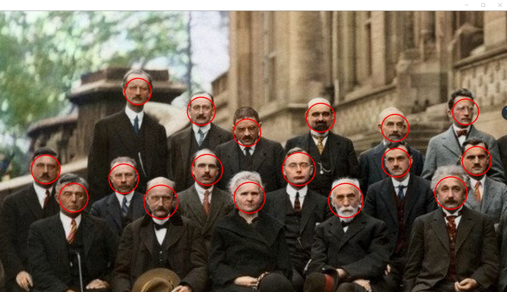
minSize=(60,60) must be added here because a personal tie will be recognized as an adult face. Through printing, you can see that only (53,53) is smaller than a normal face, so it can be filtered out through the minimum size
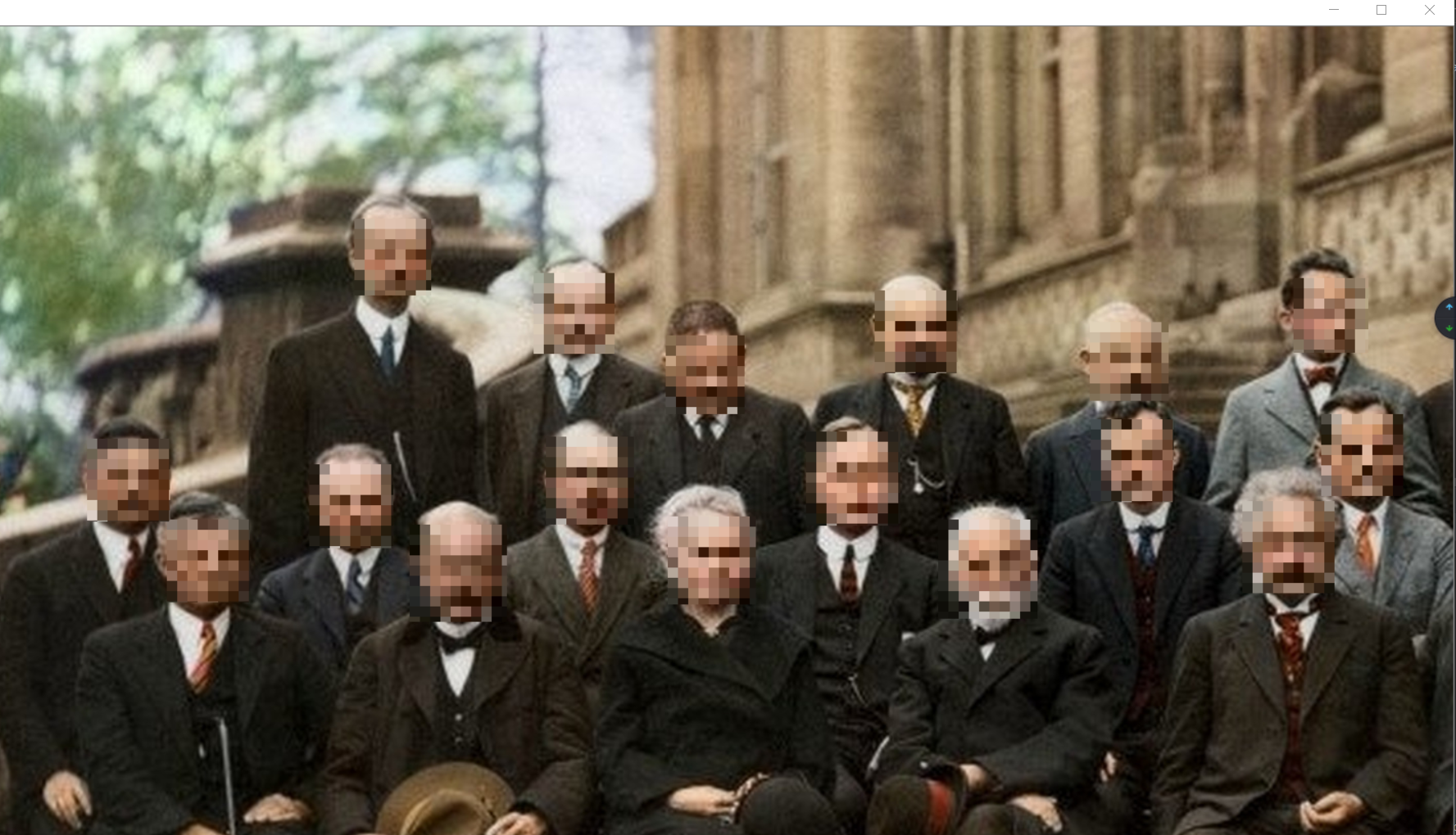
Multiple face detection + mosaic
import numpy as np
import cv2

if __name__ == '__main__':
    img = cv2.imread('./sew2.jpeg')
    gray = cv2.cvtColor(img,code=cv2.COLOR_BGR2GRAY) # Less data
    # Detailed description of face features, more than 10000 lines. The computer carries out face detection according to these features
    # According to one part, it is regarded as a face
    # Cascade classifier, detector,
    face_detector = cv2.CascadeClassifier('./haarcascade_frontalface_alt.xml')
    faces = face_detector.detectMultiScale(gray,
                                           scaleFactor=1.05,# zoom
                                           minNeighbors=10,minSize=(60,60)) # Coordinates x,y,w,h
    print(faces)
    for x,y,w,h in faces: # for loop can traverse the array!

        face = img[y:y+h,x:x+w]
        face = face[::10,::10]
        face = np.repeat(face, 10, axis=0)
        face = np.repeat(face, 10, axis=1)
        img[y:y+h,x:x+w] = face[:h,:w]
    cv2.imshow('face',img)
    cv2.waitKey(0)
    cv2.destroyAllWindows()
Face sticker
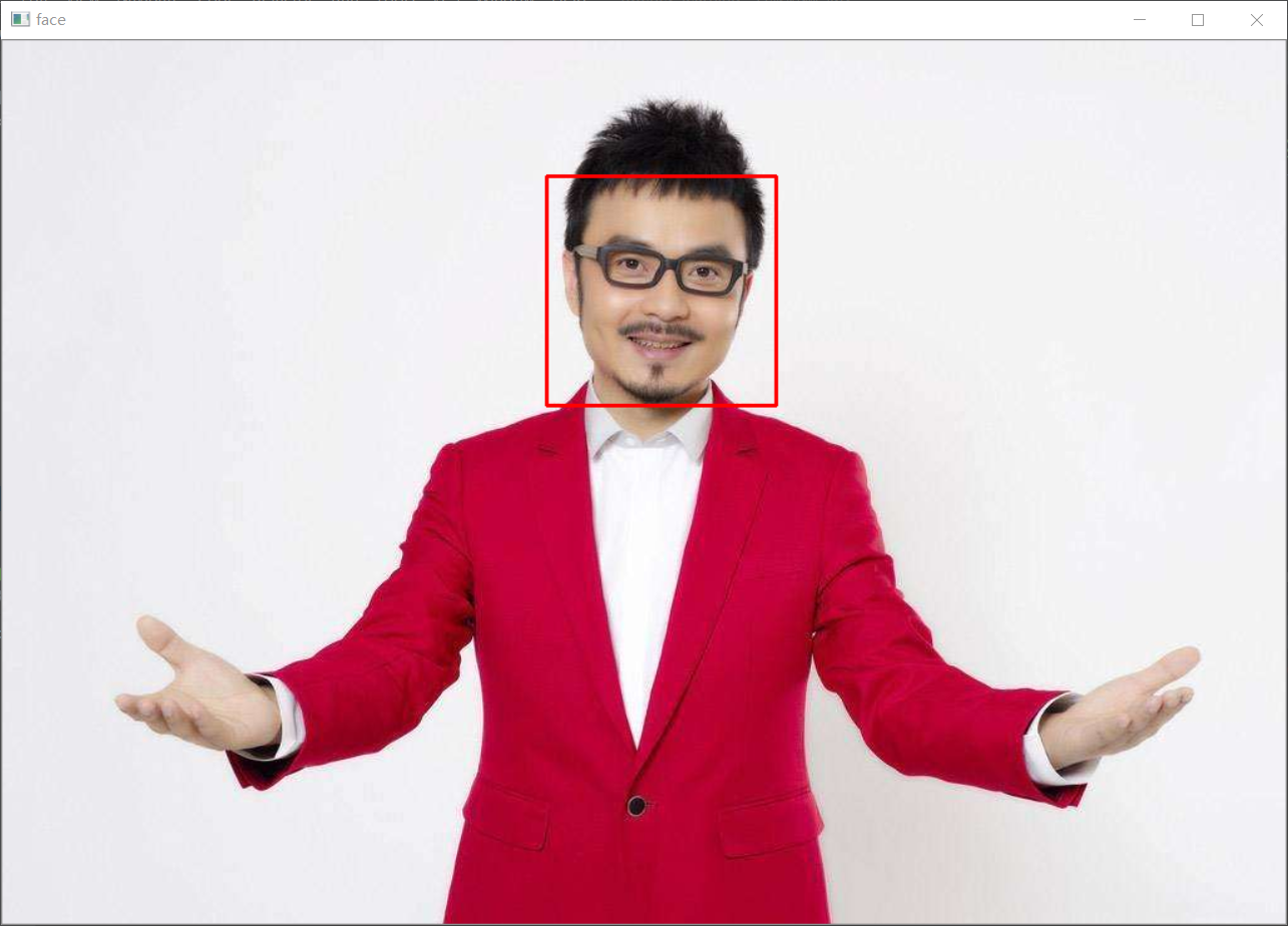
import cv2
import numpy as np

if __name__ == '__main__':
    img=cv2.imread('./han.jpeg')
    gray=cv2.cvtColor(img,code=cv2.COLOR_BGR2GRAY)
    star=cv2.imread('./star.jpg')
    # Cascade classifier, detector,
    face_detector = cv2.CascadeClassifier('./haarcascade_frontalface_alt.xml')
    faces = face_detector.detectMultiScale(gray)  # The first two are face coordinates x, y, and the last two are width and height

    for x,y,w,h in faces:
        cv2.rectangle(img, pt1=(x, y), pt2=(x + w, y + h), color=[0, 0, 255], thickness=2)
        # Rectangle pt1 is the upper left corner, pt2 is the lower right corner, and the color of color rectangle is red here. The greater the thickness value, the thicker it is
        img[y:y+h//4,x+3*w//8:x+w//4+3*w//8]=cv2.resize(star,(w//4,h//4)) # moves the coordinates to the center
    cv2.imshow('face', img)
    cv2.waitKey(0)
    cv2.destroyAllWindows()
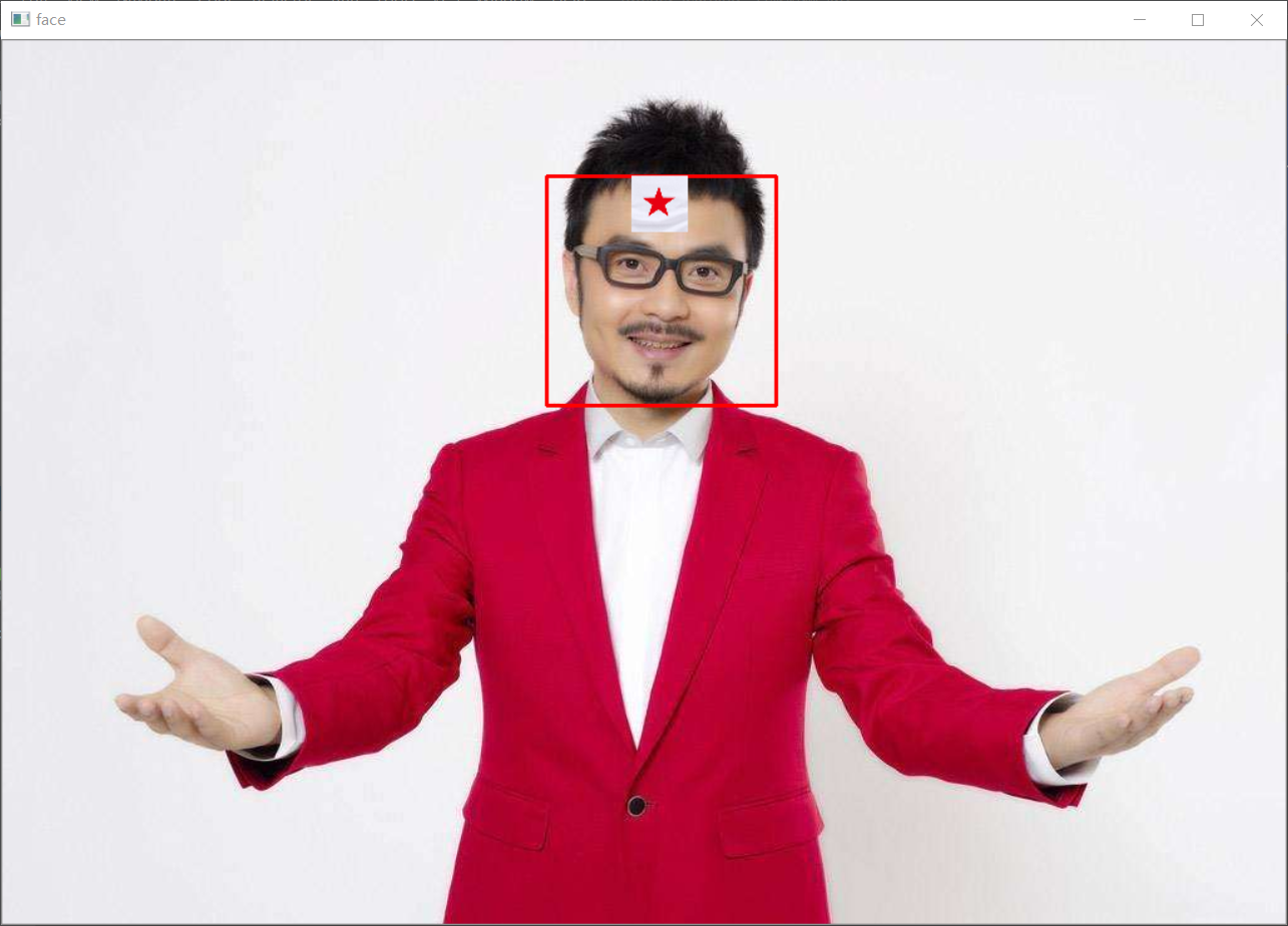
import cv2
if __name__ == '__main__':
    img = cv2.imread('./han.jpeg')
    gray = cv2.cvtColor(img, code=cv2.COLOR_BGR2GRAY)
    face_detector = cv2.CascadeClassifier('./haarcascade_frontalface_alt.xml')
    faces = face_detector.detectMultiScale(gray)
    star = cv2.imread('./star.jpg')
    for x,y,w,h in faces:
        star_s = cv2.resize(star, (w // 2, h // 2))
        w1 = w//2
        h1 = h//2
        for i in range(h1):
            for j in range(w1):#Traverse picture data
                if not (star_s[i,j] > 180).all():# gules
                    img[i+y,j+x+w//4] = star_s[i,j]
    cv2.imshow('face',img)
    cv2.waitKey(0)
    cv2.destroyAllWindows()

Hand drawn outline
import cv2
import numpy as np
if __name__ == '__main__':
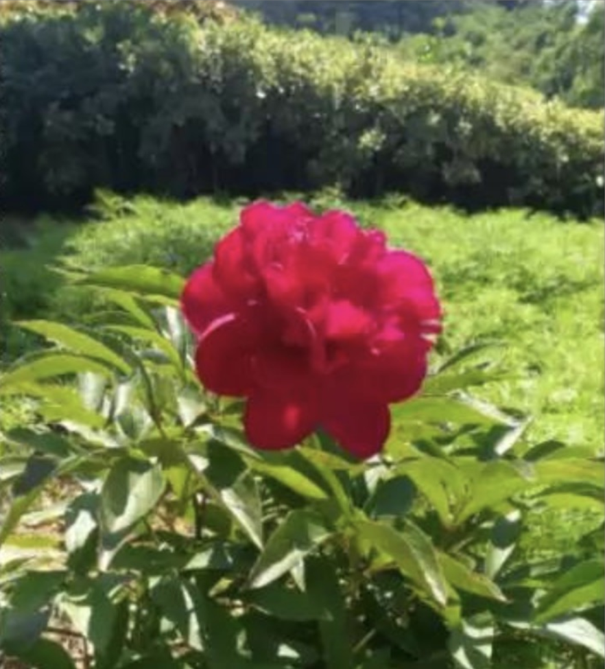
img = cv2.imread('./flower.jpg') # Blue, green and red, suitable for displaying pictures
hsv = cv2.cvtColor(img, code=cv2.COLOR_BGR2HSV) # Color space, suitable for calculation
# Contour search is performed using color values
lower_red = (156,50,50) # Light red
upper_red = (180,255,255) # oxblood red
mask = cv2.inRange(hsv, lower_red, upper_red)
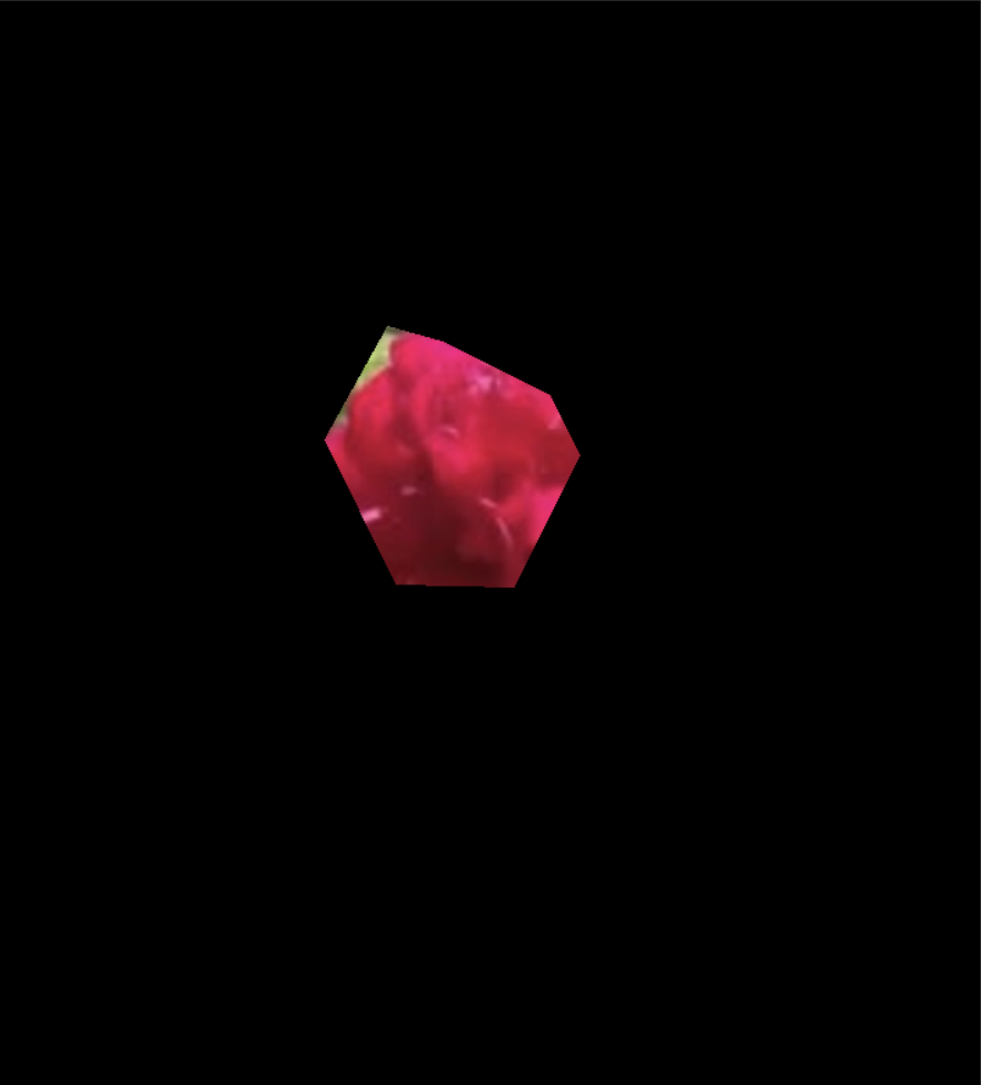
# # Hand drawn contour
h,w,c = img.shape
mask = np.zeros((h, w), dtype=np.uint8)
x_data = np.array([124, 169, 208, 285, 307, 260, 175])+110 # Abscissa
y_data = np.array([205, 124, 135, 173, 216, 311, 309])+110# Ordinate
pts = np.c_[x_data,y_data] # Abscissa and ordinate merge, point (x,y)
print(pts)
cv2.fillPoly(mask, [pts], (255)) # Draw polygons!
res = cv2.bitwise_and(img, img, mask=mask)
cv2.imshow('flower',res)
cv2.waitKey(0)
cv2.destroyAllWindows()
Find contour boundary
import cv2
import numpy as np
if __name__ == '__main__':
    dog = cv2.imread('./head.jpg')
    gray = cv2.cvtColor(dog, cv2.COLOR_BGR2GRAY)
    gray2 = cv2.GaussianBlur(gray,(5,5),0) # Gaussian smoothing
    canny = cv2.Canny(gray2,150,200)
    cv2.imshow('dog',gray)
    cv2.imshow('dog2',gray2)
    cv2.imshow('canny',canny)
    cv2.waitKey(0)
    cv2.destroyAllWindows()
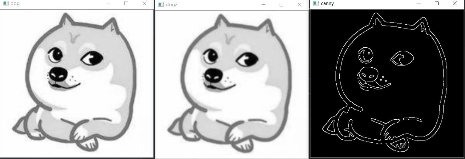
For Gaussian blur using cv2, just call Gaussian blur function in one line of code and give the size and standard deviation of Gaussian matrix:
gray2 = cv2.GaussianBlur(gray,(5,5),0) # Gaussian smoothing
Here (5, 5) means that the length and width of the Gaussian matrix are 5. When the standard deviation is 0, OpenCV will calculate it by itself according to the size of the Gaussian matrix. Generally speaking, the larger the size of Gaussian matrix, the larger the standard deviation, and the greater the degree of blur of the processed image. You can also construct your own Gaussian kernel, correlation function: CV2 GaussianKernel().
It can be used to exit the noise generated by the camera or other environment and reduce the number of remaining edges during edge extraction
cv2.Canny(src, thresh1, thresh2) performs canny edge detection
- src represents the input picture,
- thresh1 represents the minimum threshold,
- thresh2 represents the maximum threshold for further deleting edge information
Face contour replacement
import numpy as np
import cv2
if __name__ == '__main__':
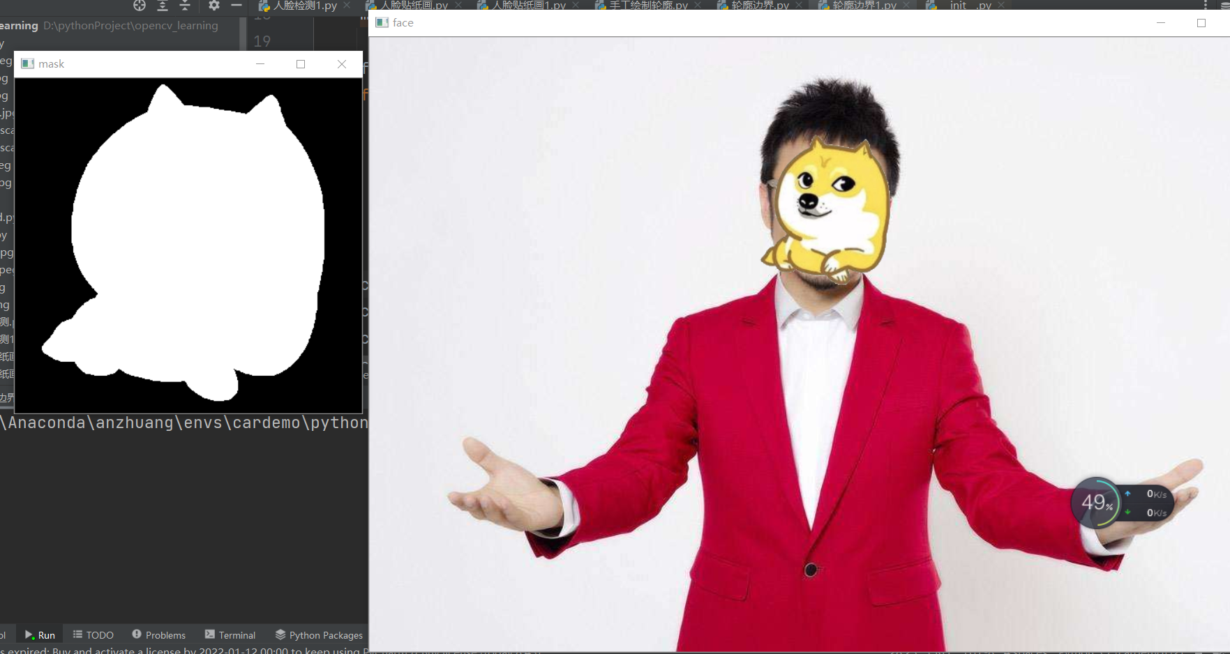
han = cv2.imread('./han.jpeg')
head = cv2.imread('./head.jpg')
face_detector = cv2.CascadeClassifier('./haarcascade_frontalface_alt.xml')
han_gray = cv2.cvtColor(han, code=cv2.COLOR_BGR2GRAY)
head_gray = cv2.cvtColor(head, code=cv2.COLOR_BGR2GRAY)
# Binarization of dog head, THRESH_OTSU will automatically set the threshold
threshold,head_binary = cv2.threshold(head_gray, 0, 255, cv2.THRESH_OTSU)
contours, hierarchy = cv2.findContours(head_binary,cv2.RETR_TREE,cv2.CHAIN_APPROX_SIMPLE)
areas = []
for contour in contours:
areas.append(cv2.contourArea(contour)) #Calculated area
areas = np.asarray(areas)
index = areas.argsort() # From small to large, the penultimate, the second largest outline
mask = np.zeros_like(head,dtype=np.uint8) # Mask mask
mask = cv2.drawContours(mask,contours,index[-2],(255,255,255),
thickness=-1)
faces = face_detector.detectMultiScale(han_gray)
for x,y,w,h in faces:
mask2 = cv2.resize(mask,(w,h))
head2 = cv2.resize(head, (w, h)) # Color picture
for i in range(h):
for j in range(w):
if (mask2[i,j] == 255).all():
han[i + y,j + x]=head2[i,j]
cv2.imshow('mask',mask)
cv2.imshow('face',han)
cv2.waitKey(0)
cv2.destroyAllWindows()
cv2.threshold(img, threshold, maxval,type)
Of which:
- Threshold is the set threshold
- maxval is the value assigned to the gray value when the gray value is greater than (or less than) the threshold
- type specifies the current binarization method
The return values are threshold and target
cv2. THRESH_ The part of binary greater than the threshold is set to 255 and the part less than the threshold is set to 0
cv2. THRESH_ BINARY_ The inv greater than the threshold value is set to 0 and the inv less than the threshold value is set to 255
cv2. THRESH_ The part of TRUNC greater than the threshold is set to threshold, and the part less than the threshold remains as it is
cv2. THRESH_ The tozero less than the threshold value is set to 0, and the greater than part remains unchanged
cv2. THRESH_ TOZERO_ The inv greater than the threshold is set to 0, and the less than part remains unchanged
In fact, there is a very important CV2 THRESH_ Otsu is an excellent algorithm for image adaptive binarization. Parameters of Otsu Otsu Otsu algorithm:
Use CV2 threshold(img, 0, 255, cv2.THRESH_OTSU )
Function CV2 Findcontours() has three parameters.
The first is the input image, the second is the contour retrieval mode, and the third is the contour approximation method.
RETR_LIST from the perspective of interpretation, this should be the simplest. It just extracts all the contours without creating any parent-child relationship.
RETR_EXTERNAL if you choose this mode, only the outermost contour will be returned, and all sub contours will be ignored.
RETR_ In this mode, ccomp returns all contours and divides them into two levels of organizational structure.
RETR_TREE this mode returns all profiles and creates a complete list of organizational structures. It will even tell you who are grandpa, Dad, son, grandson, etc
There are two return values. The first is the contour and the second is the (contour) tomographic structure
cv2.drawContours()
cv2.drawContours(image, contours, contourIdx, color, thickness=None, lineType=None, hierarchy=None, maxLevel=None, offset=None)
InputOutputArray image, / / the image to draw the outline
InputArrayOfArrays contours, / / all input contours are saved as a point vector
int contourIdx, / / specifies the number of contours to be drawn. If it is a negative number, all contours will be drawn
Const scalar & color, / / the color used to draw the outline
int thickness = 1, / / the thickness of the line drawing the contour. If it is a negative number, the interior of the contour is filled
int lineType = 8, / the connectivity of the lines that draw the outline
InputArray hierarchy = noArray(), / / optional parameters about hierarchy, which are only used when drawing partial contours
int maxLevel = INT_MAX, / / the highest level of drawing outline. This parameter is valid only when hierarchy is valid
//maxLevel=0, draw all contours belonging to the same level as the input contour, that is, the input contour and its adjacent contour
//maxLevel=1, draw all contours and their child nodes at the same level as the input contour.
//maxLevel=2, draw all contours and their child nodes at the same level as the input contour and the child nodes of the child nodes
Point offset = Point()