Catalogue of series articles
FFT
Use OpenCV to Fourier transform the image, use the FFT function available in Numpy, and some applications of Fourier transform
Correlation function: cv.dft(), cv.idft() etc.
1. Theory
Fourier transform is used to analyze the frequency characteristics of various filters. For the image, two-dimensional discrete Fourier transform (DFT) is used to calculate the frequency domain. Fast Fourier transform (FFT) algorithm is used to calculate DFT. Details of these can be found in any textbook on image processing or signal processing. See the additional resources section.
sinusoidal signal x ( t ) = A sin ( 2 π f t ) x(t)=A \sin (2 \pi f t) x(t)=Asin(2 π ft), we can say that f is the frequency of the signal. If we observe its frequency domain, we can see a peak in F. If the signal is sampled to form a discrete signal, we get the same frequency domain, but the period is (− π, π] or [0,2 π) (in N-point DFT, (0,N)). You can think of an image as a signal sampled in two directions. Fourier transform is performed in X and Y directions to obtain the frequency representation of the image.
More intuitively, for a sinusoidal signal, if the amplitude changes so fast in a short time, you can say it is a high-frequency signal. If the change is slow, it is a low-frequency signal. You can extend the same idea to the image. Where does the amplitude vary greatly in the image? At edge points, or noise. So we can say that edge and noise are the high-frequency content in the image. If the amplitude changes little, it is a low-frequency component. (some links are added to the additional resource), which intuitively explains the example of frequency conversion).
Now let's look at how to find the Fourier transform.
2. Fourier transform (Numpy)
First, we'll see how to use numpy for Fourier transform. Numpy has an FFT package to do this. Np. fft. FFT 2 () provides us with the frequency transformation of a complex array. Its first parameter is the input image, that is, gray. The second parameter is optional and determines the size of the output array. If it is larger than the size of the input image, the input image is filled with zeros before FFT calculation. If it is smaller than the input image, the input image will be cropped. If no parameters are passed in, the output array will be the same size as the input array.
Now once you get the result, the zero frequency component (DC component) will be in the upper left corner. If you want to center it, you need to move N/2 in both directions. This is just by the function * * NP fft. Fftshift() * * complete. (this analysis is more intuitive). Once you find the frequency transformation, you can find the amplitude spectrum.
import cv2 as cv
import numpy as np
from matplotlib import pyplot as plt
img = cv.imread('messi5.jpg',0)
f = np.fft.fft2(img)
fshift = np.fft.fftshift(f)
magnitude_spectrum = 20*np.log(np.abs(fshift))
plt.subplot(121),plt.imshow(img, cmap = 'gray')
plt.title('Input Image'), plt.xticks([]), plt.yticks([])
plt.subplot(122),plt.imshow(magnitude_spectrum, cmap = 'gray')
plt.title('Magnitude Spectrum'), plt.xticks([]), plt.yticks([])
plt.show()
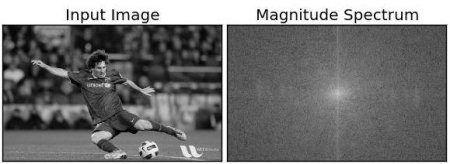
Look, you can see more white areas in the center, which represent low-frequency components.
So you implemented the frequency transformation. Now you can do some operations in the frequency domain, such as high pass filtering and image reconstruction, or vice versa. To do this, you only need to shield the low frequency through a rectangular window with a size of 60x60. Then use NP fft. Ifftshift() performs inverse transformation to make the DC component appear in the upper left corner again. Then use NP The ifft2() function finds the inverse FFT. The result is a complex number. You can take its absolute value.
rows, cols = img.shape
crow,ccol = rows//2 , cols//2
fshift[crow-30:crow+31, ccol-30:ccol+31] = 0
f_ishift = np.fft.ifftshift(fshift)
img_back = np.fft.ifft2(f_ishift)
img_back = np.real(img_back)
plt.subplot(131),plt.imshow(img, cmap = 'gray')
plt.title('Input Image'), plt.xticks([]), plt.yticks([])
plt.subplot(132),plt.imshow(img_back, cmap = 'gray')
plt.title('Image after HPF'), plt.xticks([]), plt.yticks([])
plt.subplot(133),plt.imshow(img_back)
plt.title('Result in JET'), plt.xticks([]), plt.yticks([])
plt.show()
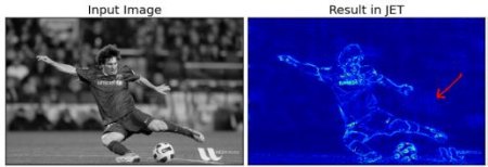
The results show that the high pass filter is an edge extraction operation. We mentioned this in the previous image gradient chapter. This also shows that most of the components in the image are low-frequency parts. Anyway, we have seen how to find DFT, IDFT, etc. in Numpy. Now let's see how to do it in OpenCV.
If you look closely at the results, especially the last JET color image, you can see some components (an example I marked with a red arrow). It shows some corrugated structures, which is called ringing effect. This is because we use a rectangular window as a mask. This mask is converted to a sin shape, which causes this problem. Therefore, rectangular windows are not used for filtering. A better choice is the Gaussian window.
3. Fourier transform (Opencv)
OpenCV provides cv.dft() and cv.idft() Function. It returns the same result as before, but with two channels. The first channel is the real part of the result, and the second channel is the imaginary part of the result. The input image should be converted to NP float32. We'll see how to do it.
import numpy as np
import cv2 as cv
from matplotlib import pyplot as plt
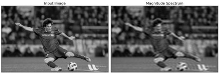
img = cv.imread('messi5.jpg',0)
dft = cv.dft(np.float32(img),flags = cv.DFT_COMPLEX_OUTPUT)
dft_shift = np.fft.fftshift(dft)
magnitude_spectrum = 20*np.log(cv.magnitude(dft_shift[:,:,0],dft_shift[:,:,1]))
plt.subplot(121),plt.imshow(img, cmap = 'gray')
plt.title('Input Image'), plt.xticks([]), plt.yticks([])
plt.subplot(122),plt.imshow(magnitude_spectrum, cmap = 'gray')
plt.title('Magnitude Spectrum'), plt.xticks([]), plt.yticks([])
plt.show()
Note: you can also use cv.cartToPolar() , it returns both amplitude and phase
Now we're going to do the inverse DFT. In the previous session, we created an HPF (high pass filter). This time, we will see how to delete the high-frequency content in the image, that is, we apply LPF (low-pass filter). It actually blurs the image. To do this, we first create a mask with 1 in the low-frequency part and 0 in the high-frequency part.
rows, cols = img.shape
crow,ccol = rows/2 , cols/2
# create a mask first, center square is 1, remaining all zeros
mask = np.zeros((rows,cols,2),np.uint8)
mask[crow-30:crow+30, ccol-30:ccol+30] = 1
# apply mask and inverse DFT
fshift = dft_shift*mask
f_ishift = np.fft.ifftshift(fshift)
img_back = cv.idft(f_ishift)
img_back = cv.magnitude(img_back[:,:,0],img_back[:,:,1])# Calculated amplitude
plt.subplot(121),plt.imshow(img, cmap = 'gray')
plt.title('Input Image'), plt.xticks([]), plt.yticks([])
plt.subplot(122),plt.imshow(img_back, cmap = 'gray')
plt.title('Magnitude Spectrum'), plt.xticks([]), plt.yticks([])
plt.show()
about cv.magnitude , which is used to calculate the size of two-dimensional vector. That is, for vectors
(
x
,
y
)
(x,y)
(x,y), calculate its size (modulus):
dst
(
I
)
=
x
(
I
)
2
+
y
(
I
)
2
\texttt{dst} (I) = \sqrt{\texttt{x}(I)^2 + \texttt{y}(I)^2}
dst(I)=x(I)2+y(I)2
result:
4. DFT performance optimization
DFT calculations perform better for some array sizes. When the array size is a power of 2, it is the fastest. The processing efficiency is also quite high for arrays with the product of sizes 2, 3 and 5. Therefore, if you are worried about the performance of your code, you can change the size of the array to any optimal size (by filling in zeros) before finding the DFT. For OpenCV, you must manually fill in zeros. But for Numpy, if you specify the new size of FFT calculation, it will automatically fill in zeros for you.
So how to find the optimal size? OpenCV provides a function cv getOptimalDFTSize(). cvt .dft() and NP fft. Both fft2 () apply. Let's use the IPython magic command timeit to check their performance.
In [16]: img = cv.imread('messi5.jpg',0)
In [17]: rows,cols = img.shape
In [18]: print("{} {}".format(rows,cols))
342 548
In [19]: nrows = cv.getOptimalDFTSize(rows)
In [20]: ncols = cv.getOptimalDFTSize(cols)
In [21]: print("{} {}".format(nrows,ncols))
360 576
Look, the size (342548) is changed to (360576). Now let's fill it with zeros (for OpenCV) and find out their DFT computing performance. You can do this by creating a new larger all zero array and copying the data to it, or using cv copyMakeBorder().
nimg = np.zeros((nrows,ncols))
nimg[:rows,:cols] = img
perhaps
right = ncols - cols
bottom = nrows - rows
bordertype = cv.BORDER_CONSTANT #just to avoid line breakup in PDF file
nimg = cv.copyMakeBorder(img,0,bottom,0,right,bordertype, value = 0)
Now let's compare the DFT performance of Numpy function:
In [22]: %timeit fft1 = np.fft.fft2(img)
10 loops, best of 3: 40.9 ms per loop
In [23]: %timeit fft2 = np.fft.fft2(img,[nrows,ncols])
100 loops, best of 3: 10.4 ms per loop
It can be seen that it is four times faster. Now we'll do the same with the OpenCV function.
In [24]: %timeit dft1= cv.dft(np.float32(img),flags=cv.DFT_COMPLEX_OUTPUT)
100 loops, best of 3: 13.5 ms per loop
In [27]: %timeit dft2= cv.dft(np.float32(nimg),flags=cv.DFT_COMPLEX_OUTPUT)
100 loops, best of 3: 3.11 ms per loop
It can be seen that it is four times faster. You can also see that the OpenCV function is about three times faster than the Numpy function. This can also be used to test inverse FFT, which is left for you to practice.
5. Why is Laplacian a high pass filter?
Similar questions were also asked in a forum. The question is, why is Laplacian a high pass filter? Why is sobel a high pass filter? Wait. The answer to the first question is related to Fourier transform. Laplace transform is performed on the larger Fourier transform. analysis:
import cv2 as cv
import numpy as np
from matplotlib import pyplot as plt
# simple averaging filter without scaling parameter
mean_filter = np.ones((3,3))
# creating a gaussian filter
x = cv.getGaussianKernel(5,10)
gaussian = x*x.T
# different edge detecting filters
# scharr in x-direction
scharr = np.array([[-3, 0, 3],
                   [-10,0,10],
                   [-3, 0, 3]])
# sobel in x direction
sobel_x= np.array([[-1, 0, 1],
                   [-2, 0, 2],
                   [-1, 0, 1]])
# sobel in y direction
sobel_y= np.array([[-1,-2,-1],
                   [0, 0, 0],
                   [1, 2, 1]])
# laplacian
laplacian=np.array([[0, 1, 0],
                    [1,-4, 1],
                    [0, 1, 0]])
filters = [mean_filter, gaussian, laplacian, sobel_x, sobel_y, scharr]
filter_name = ['mean_filter', 'gaussian','laplacian', 'sobel_x', \
                'sobel_y', 'scharr_x']
fft_filters = [np.fft.fft2(x) for x in filters]
fft_shift = [np.fft.fftshift(y) for y in fft_filters]
mag_spectrum = [np.log(np.abs(z)+1) for z in fft_shift]
for i in range(6):
    plt.subplot(2,3,i+1),plt.imshow(mag_spectrum[i],cmap = 'gray')
    plt.title(filter_name[i]), plt.xticks([]), plt.yticks([])
plt.show()
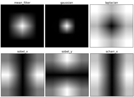
From the image, you can see the frequency region of each kernel block and the region it passes through. From this information, we can know why each kernel is HPF or LPF
Extended data
- An Intuitive Explanation of Fourier Theory by Steven Lehar
- Fourier Transform at HIPR
- What does frequency domain denote in case of images?
reference resources: https://docs.opencv.org/4.5.2/dd/dc4/tutorial_py_table_of_contents_transforms.html