Original Link:http://www.juzicode.com/opencv-python-image-gradient
Return to the Opencv-Python tutorial
Gaussian smoothing, bilateral smoothing And Mean Smoothing, Median Smoothing The smoothing described can be seen as a "low-pass filter" of the image, which filters out the "high frequency" part of the image to make it look smoother, while the image gradient can be thought of as a "high-pass filter" of the image, which filters out the low frequency part of the image in order to highlight the abrupt parts of the image. Morphological Transform~On/Off Operation, Black Cap, Morphological Gradient, Shape Ex We have also touched on image gradients in the article. Today we will continue to introduce several methods for calculating image gradients.
1,Sobel
The Sobel 3 x 3 kernels are shown in the following figure. From the kernels you can see that calculating the Sobel gradient has a gradient in both X and Y directions:
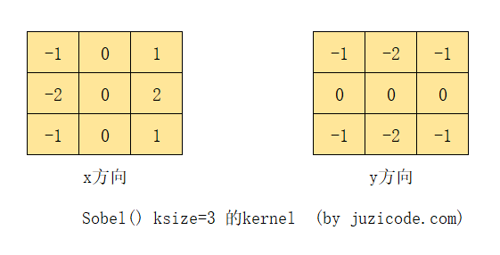
For example, in the Obel kernels of size 3 by 3 above, the x-direction gradient is 2 times the right pixel value of the point, 2 times the right upper and right lower pixel value, 2 times the subtraction of the left pixel value, and the sum of the left upper and left lower pixel value. The gradient value of this point is independent of itself, only related to the left and right pixel values, and the y-direction gradient is related to the upper and lower pixel values.
Interface form:
dst = cv2.Sobel(src, ddepth, dx, dy[, dst[, ksize[, scale[, delta[, borderType]]]]])
- Parameter meaning:
- src: source image;
- ddepth: target image depth;
- Derivative order in dx:x direction;
- Derivative order in dy:y direction;
- dst: target image;
- ksize:kernel size, which indicates in the documentation that it must be one of 1,3,5,7, but the experiment yields positive and odd numbers that should be less than 31; if -1 means scharr filter;
- scale: scale, default is 1;
- delta: overlay value, default is 0;
- borderType: Boundary fill type;
In the example below, first set dx=1, dy=0 to calculate the gradient in the x direction, then set dy=1, and dx=0 to calculate the gradient in the y direction. To avoid the saturation operation, dtype sets CV_16S higher than the source image data type CV_8U, then converts the result back to the CV_8U(np.unit8) type with convertScaleAbs(), and finally addWeighted() to add the gradient graph in the x and y directions.
import matplotlib.pyplot as plt
import cv2
print('VX Public Number: Orange code / juzicode.com')
print('cv2.__version__:',cv2.__version__)
plt.rc('font',family='Youyuan',size='9')

img_src = cv2.imread('..\\samples\\data\\sudoku.png' ,cv2.IMREAD_GRAYSCALE)
grad_x = cv2.Sobel(img_src, cv2.CV_16S, 1, 0, ksize=3)
grad_y = cv2.Sobel(img_src, cv2.CV_16S, 0, 1, ksize=3)

abs_grad_x = cv2.convertScaleAbs(grad_x)
abs_grad_y = cv2.convertScaleAbs(grad_y)
grad = cv2.addWeighted(abs_grad_x, 0.5, abs_grad_y, 0.5, 0)

fig,ax = plt.subplots(2,2)
ax[0,0].set_title('Original Map(juzicode.com)')
ax[0,0].imshow(img_src ,cmap = 'gray')
ax[0,1].set_title('abs_grad_x')
ax[0,1].imshow(abs_grad_x,cmap = 'gray')
ax[1,0].set_title('abs_grad_y')
ax[1,0].imshow(abs_grad_y,cmap = 'gray')
ax[1,1].set_title('grad x+y')
ax[1,1].imshow(grad,cmap = 'gray')
ax[0,0].axis('off');ax[0,1].axis('off');ax[1,0].axis('off');ax[1,1].axis('off')#Turn off axis display
plt.show()
Run result:
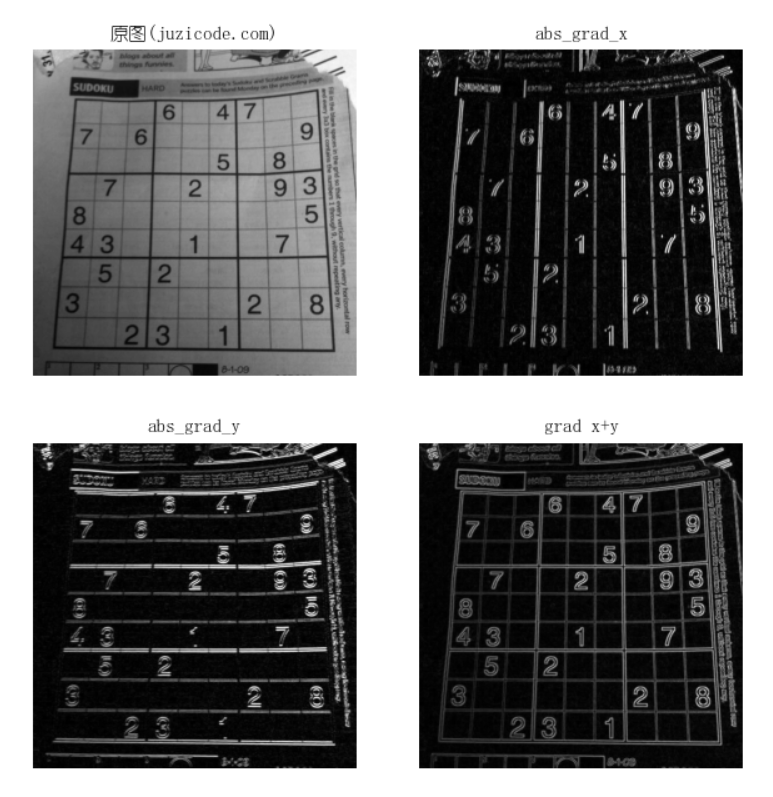
The upper right corner of the above image is a gradient change along the x direction, the lower left is a gradient change along the y direction, and the lower right corner is a combination of half the weight of the two. From the combined gradient image, you can see that the edges of the original image's checkerboard lines and numbers become brighter, while the continuous areas of brightness between the blank and the numbers become darker, and finally the edges are highlighted.Fruit.
If dx and dy are both set to 1:grad_x_y = cv2.Sobel(img_src, cv2.CV_16S, 1, 1, ksize=3), let's see how this works:
import matplotlib.pyplot as plt
import cv2
print('VX Public Number: Orange code / juzicode.com')
print('cv2.__version__:',cv2.__version__)
plt.rc('font',family='Youyuan',size='9')

img_src = cv2.imread('..\\samples\\data\\sudoku.png' ,cv2.IMREAD_GRAYSCALE)
grad_x = cv2.Sobel(img_src, cv2.CV_16S, 1, 0, ksize=3)
grad_y = cv2.Sobel(img_src, cv2.CV_16S, 0, 1, ksize=3)
abs_grad_x = cv2.convertScaleAbs(grad_x)
abs_grad_y = cv2.convertScaleAbs(grad_y)
grad = cv2.addWeighted(abs_grad_x, 0.5, abs_grad_y, 0.5, 0)
#Finding both x and y direction gradients
grad_x_y = cv2.Sobel(img_src, cv2.CV_16S, 1, 1, ksize=3)
abs_grad_x_y = cv2.convertScaleAbs(grad_x_y)

fig,ax = plt.subplots(2,2)
ax[0,0].set_title('Original Map(juzicode.com)')
ax[0,0].imshow(img_src ,cmap = 'gray')
ax[0,1].set_title('abs_grad_x')
ax[0,1].imshow(abs_grad_x,cmap = 'gray')
ax[1,0].set_title('grad_x+y')
ax[1,0].imshow(grad,cmap = 'gray')
ax[1,1].set_title('abs_grad_dx_dy=1')
ax[1,1].imshow(abs_grad_x_y,cmap = 'gray')
ax[0,0].axis('off');ax[0,1].axis('off');ax[1,0].axis('off');ax[1,1].axis('off')#Turn off axis display
plt.show() 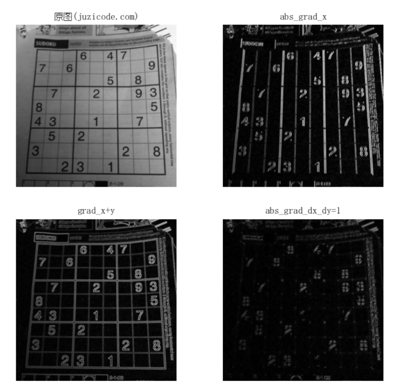
As you can see from the running results, when dx and dy are set to the image at the bottom right of the above image at the same time, the gradients of horizontal and vertical lines in the board disappear, where dx and dy are both 1 indicating a relationship with each other, and can only be detected if both x and y have gradients.
The next example is setting different ksize:
import matplotlib.pyplot as plt
import cv2
print('VX Public Number: Orange code / juzicode.com')
print('cv2.__version__:',cv2.__version__)
plt.rc('font',family='Youyuan',size='9')

img_src = cv2.imread('..\\samples\\data\\sudoku.png' ,cv2.IMREAD_GRAYSCALE)
print(img_src.shape)
grad_x_ksize1 = cv2.Sobel(img_src, cv2.CV_16S, 1, 0, ksize=1)
grad_x_ksize3 = cv2.Sobel(img_src, cv2.CV_16S, 1, 0, ksize=3)
grad_x_ksize5 = cv2.Sobel(img_src, cv2.CV_16S, 1, 0, ksize=5)
#Setting different ksize values
abs_grad_x_ksize1 = cv2.convertScaleAbs(grad_x_ksize1)
abs_grad_x_ksize3 = cv2.convertScaleAbs(grad_x_ksize3)
abs_grad_x_ksize5 = cv2.convertScaleAbs(grad_x_ksize5)
#display
fig,ax = plt.subplots(2,2)
ax[0,0].set_title('Original Map(juzicode.com)')
ax[0,0].imshow(img_src ,cmap = 'gray')
ax[0,1].set_title('abs_grad_x_ksize=1')
ax[0,1].imshow(abs_grad_x_ksize1,cmap = 'gray')
ax[1,0].set_title('abs_grad_x_ksize=3')
ax[1,0].imshow(abs_grad_x_ksize3,cmap = 'gray')
ax[1,1].set_title('abs_grad_x_ksize=5')
ax[1,1].imshow(abs_grad_x_ksize5,cmap = 'gray')
ax[0,0].axis('off');ax[0,1].axis('off');ax[1,0].axis('off');ax[1,1].axis('off')#Turn off axis display
plt.show() 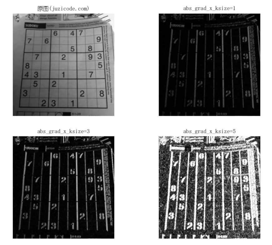
In the example above, ksize is set to 1,3,5 in turn, and the larger the value of ksize, the more the gradient information is presented.
Let's set the derivative order differently. Take dx in the x direction for example. When ksize=5, set the dx to be 1,2,3. Note that the value of dx is less than ksize:
import matplotlib.pyplot as plt
import cv2
print('VX Public Number: Orange code / juzicode.com')
print('cv2.__version__:',cv2.__version__)
plt.rc('font',family='Youyuan',size='9')

img_src = cv2.imread('..\\samples\\data\\sudoku.png' ,cv2.IMREAD_GRAYSCALE)
#Same ksize, different dx
grad_order1 = cv2.Sobel(img_src, cv2.CV_16S, 1, 0, ksize=5)
grad_order2 = cv2.Sobel(img_src, cv2.CV_16S, 2, 0, ksize=5)
grad_order3 = cv2.Sobel(img_src, cv2.CV_16S, 3, 0, ksize=5)
abs_grad_order1 = cv2.convertScaleAbs(grad_order1)
abs_grad_order2 = cv2.convertScaleAbs(grad_order2)
abs_grad_order3 = cv2.convertScaleAbs(grad_order3)

fig,ax = plt.subplots(2,2)
ax[0,0].set_title('Original Map(juzicode.com)')
ax[0,0].imshow(img_src ,cmap = 'gray')
ax[0,1].set_title('abs_grad_order1')
ax[0,1].imshow(abs_grad_order1,cmap = 'gray')
ax[1,0].set_title('abs_grad_order2')
ax[1,0].imshow(abs_grad_order2,cmap = 'gray')
ax[1,1].set_title('abs_grad_order3')
ax[1,1].imshow(abs_grad_order3,cmap = 'gray')
ax[0,0].axis('off');ax[0,1].axis('off');ax[1,0].axis('off');ax[1,1].axis('off')#Turn off axis display
plt.show() 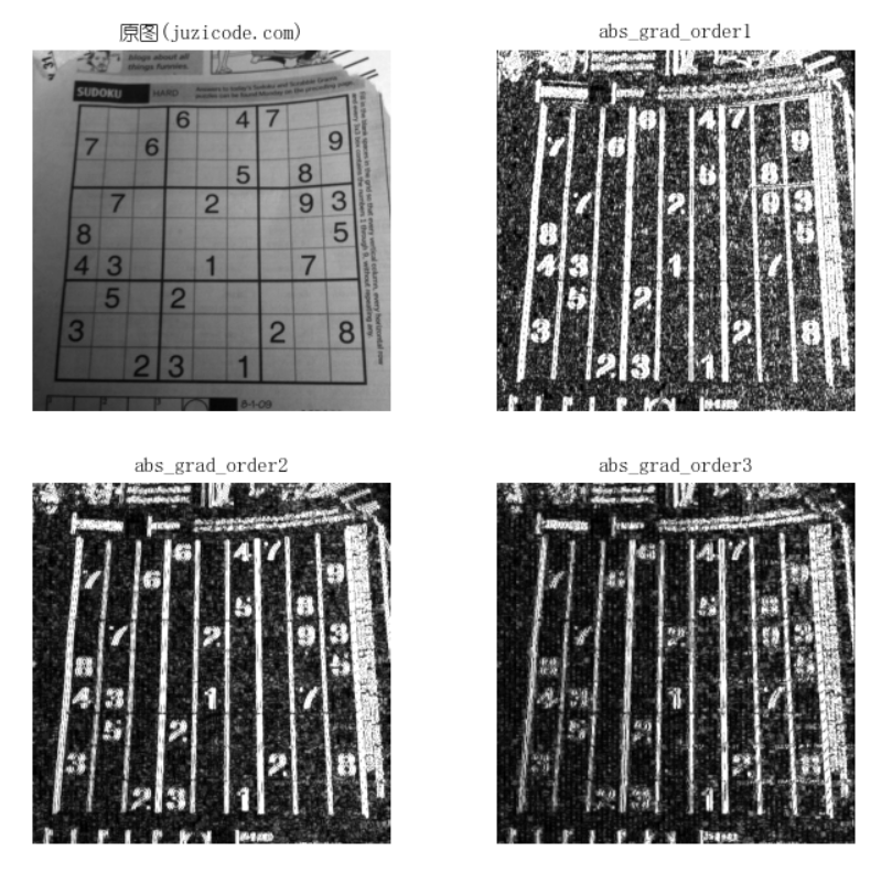
You can see from the running results that the smaller the dx value, the more detail of the gradient under the same ksize.
2,Scharr
Sobel's results are not very accurate when the kernels are 3 x 3 in size. Scharr kernel s shown in the following figure are often used for more accurate calculations:
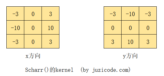
The Scharr transformation can be seen as a Sobel transformation using the Scharr kernel, which is an improved Sobel transformation and calculates gradients separately from the x and y directions.
Interface form:
dst = cv2.Scharr(src, ddepth, dx, dy[, dst[, scale[, delta[, borderType]]]])
- Parameter meaning:
- src: source image;
- ddepth: target image depth;
- Derivative order in dx:x direction;
- Derivative order in dy:y direction;
- dst: target image;
- scale: scale, default is 1;
- delta: overlay value, default is 0;
- borderType: Boundary fill type;
Note that Scharr() does not have a ksize parameter because the size of the Scharr kernel is fixed to 3 by 3.
The following example is similar to the previous image gradient calculation using Sobel(), where the x-direction gradient is calculated, then the y-direction gradient is calculated, and then the total gradient image is weighted:
import matplotlib.pyplot as plt
import cv2
print('VX Public Number: Orange code / juzicode.com')
print('cv2.__version__:',cv2.__version__)
plt.rc('font',family='Youyuan',size='9')

img_src = cv2.imread('..\\samples\\data\\sudoku.png' ,cv2.IMREAD_GRAYSCALE)
grad_x = cv2.Scharr(img_src,cv2.CV_16S,1,0)
grad_y = cv2.Scharr(img_src,cv2.CV_16S,0,1)
abs_grad_x = cv2.convertScaleAbs(grad_x)
abs_grad_y = cv2.convertScaleAbs(grad_y)
grad = cv2.addWeighted(abs_grad_x, 0.5, abs_grad_y, 0.5, 0)

fig,ax = plt.subplots(2,2)
ax[0,0].set_title('Original Map(juzicode.com)')
ax[0,0].imshow(img_src ,cmap = 'gray')
ax[0,1].set_title('abs_grad_x')
ax[0,1].imshow(abs_grad_x,cmap = 'gray')
ax[1,0].set_title('abs_grad_y')
ax[1,0].imshow(abs_grad_y,cmap = 'gray')
ax[1,1].set_title('grad-x+y')
ax[1,1].imshow(grad,cmap = 'gray')
ax[0,0].axis('off');ax[0,1].axis('off');ax[1,0].axis('off');ax[1,1].axis('off')
plt.show()
Run result:
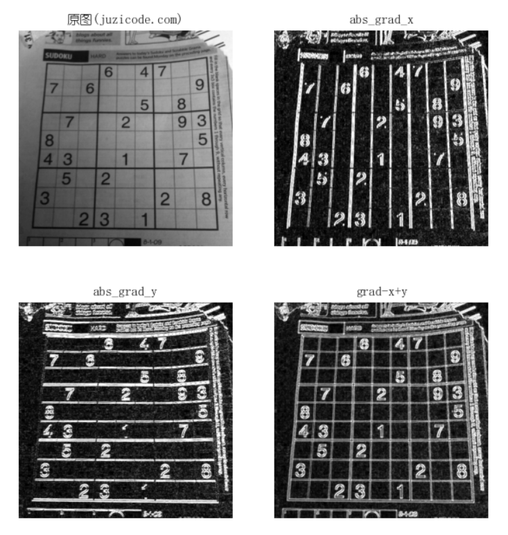
It is important to note that when calculating the Scharr gradient, dx and dy must satisfy the following relationships, or an exception will be thrown:
CV_Assert( dx >= 0 && dy >= 0 && dx+dy == 1 )
That is, only single-direction gradients in either x or y direction can be found at a time, and only first-order gradients can be found, unlike dx or dy in Sobel(), which can be set to larger values to calculate higher-order gradients.
3,Laplacian
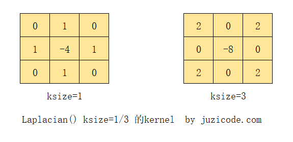
The Laplacian transformation is to derive the second derivative of the image. In the following figure, there are two kernel s of 3 x 3 size, where ksize is the name of the input of Laplacian():
The Laplacian() transformation does not require a gradient to be calculated in the X and y directions of the image. You can also see from the two kernel s in the figure above that their x and y directions are symmetrical.
In the Laplacian() transformation, ksize must be a positive and odd number less than 31, but when ksize equals 1, the size of the kernels is not 1, but the actual size is still 3 x 3, which shows from the source that when ksize=1, it is actually a 3 x 3 kernel with 9 elements:
    if( ksize == 1 || ksize == 3 ){
        float K[2][9] = {
            { 0, 1, 0, 1, -4, 1, 0, 1, 0 }, //kernel at ksize==1
            { 2, 0, 2, 0, -8, 0, 2, 0, 2 }  //kernel at ksize==3
        };
        Mat kernel(3, 3, CV_32F, K[ksize == 3]);
        ......
    }
Interface form:
dst = cv2.Laplacian(src, ddepth[, dst[, ksize[, scale[, delta[, borderType]]]]])
- Parameter meaning:
- src: source image;
- ddepth: target image depth;
- dst: target image;
- ksize: Kernel size, positive and odd numbers less than 31; if 1 is still a 3*3 kernel;
- scale: scale, default is 1;
- delta: overlay value, default is 0;
- borderType: Boundary fill type;
There is no dx or dy parameter in the Laplacian transformation because Laplacian is the second derivative of the image.
The following example shows the different ksize s in Laplacian and the comparison with obel:
import matplotlib.pyplot as plt
import cv2
print('VX Public Number: Orange code / juzicode.com')
print('cv2.__version__:',cv2.__version__)
plt.rc('font',family='Youyuan',size='9')

img_src = cv2.imread('..\\samples\\data\\sudoku.png' ,cv2.IMREAD_GRAYSCALE)
#Laplacian
grad_lap = cv2.Laplacian(img_src,cv2.CV_16S,ksize=1)
abs_grad_lap1 = cv2.convertScaleAbs(grad_lap)
grad_lap = cv2.Laplacian(img_src,cv2.CV_16S,ksize=3)
abs_grad_lap3 = cv2.convertScaleAbs(grad_lap)
grad_lap = cv2.Laplacian(img_src,cv2.CV_16S,ksize=5)
abs_grad_lap5 = cv2.convertScaleAbs(grad_lap)
#Second Order Sobel
grad_x = cv2.Sobel(img_src, cv2.CV_16S, 2, 0, ksize=3)
grad_y = cv2.Sobel(img_src, cv2.CV_16S, 0, 2, ksize=3)
abs_grad_x = cv2.convertScaleAbs(grad_x)
abs_grad_y = cv2.convertScaleAbs(grad_y)
abs_grad_sobel = cv2.addWeighted(abs_grad_x, 0.5, abs_grad_y, 0.5, 0)
#display
fig,ax = plt.subplots(2,3)
ax[0,0].set_title('Original Map(juzicode.com)')
ax[0,0].imshow(img_src ,cmap = 'gray')
ax[0,1].set_title('abs_grad_sobel')
ax[0,1].imshow(abs_grad_sobel,cmap = 'gray')
ax[1,0].set_title('abs_grad_lap1')
ax[1,0].imshow(abs_grad_lap1,cmap = 'gray')
ax[1,1].set_title('abs_grad_lap3')
ax[1,1].imshow(abs_grad_lap3,cmap = 'gray')
ax[1,2].set_title('abs_grad_lap5')
ax[1,2].imshow(abs_grad_lap5,cmap = 'gray')
ax[0,0].axis('off');ax[0,1].axis('off');ax[0,2].axis('off')#Turn off axis display
ax[1,0].axis('off');ax[1,1].axis('off');ax[1,2].axis('off')
plt.show()
Run result:
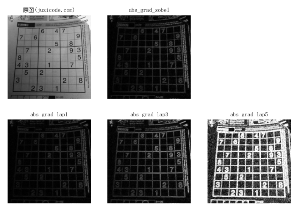
It can be seen from the running results that the larger the ksize in Laplacian(), the richer the gradient information, which is the same as the Sobel transformation. In addition, the second-order Sobel transformation and the Laplacian transformation obtain more distinct gradient information than the Laplacian transformation when the ksize is the same.