This paper mainly refers to:
PCT Get started;
International application of the PCT methods
This paper mainly introduces the R package PCT, whose goal is to improve the accessibility and repeatability of the data generated by the dependency to cycle too (PCT), which is hosted on www.pct.bike.
The bicycle use data study (dependency ot cycle - PCT) in England and Wales is a good tool to study bicycles, slow traffic and sustainable transportation. PCT An open source online system for sustainable transportation planning The method and motivation of the project are introduced in detail.
A major motivation behind the project is to make transport evidence more accessible and encourage evidence-based transport policies. PCT's code base is publicly available (see github.com/npct). However, the code hosted there is not easy to run or copy, which is where this package is used: it provides fast access to PCT basic data and enables some key results to be copied quickly. Its development is mainly for educational purposes (including the upcoming PCT training course), but it may be useful for people to develop on the basis of these methods, such as creating a bicycle scene in their town / city / area.
In a word, if you want to understand the working principle of PCT, reproduce some of its results, and build a bicycle use scenario to inform the traffic policy supporting cycling in cities around the world, this R package is very suitable for learning
1. Install the loading package
# install.packages("pct")
library(pct)
2. Data import
Get and copy some data sets from PCT package, based on an example of San Diego. This paper shows how to use the package to estimate the bicycle potential of other cities.
The code of this data can be processed or obtained through this file pctSantiago.
head(santiago_od)
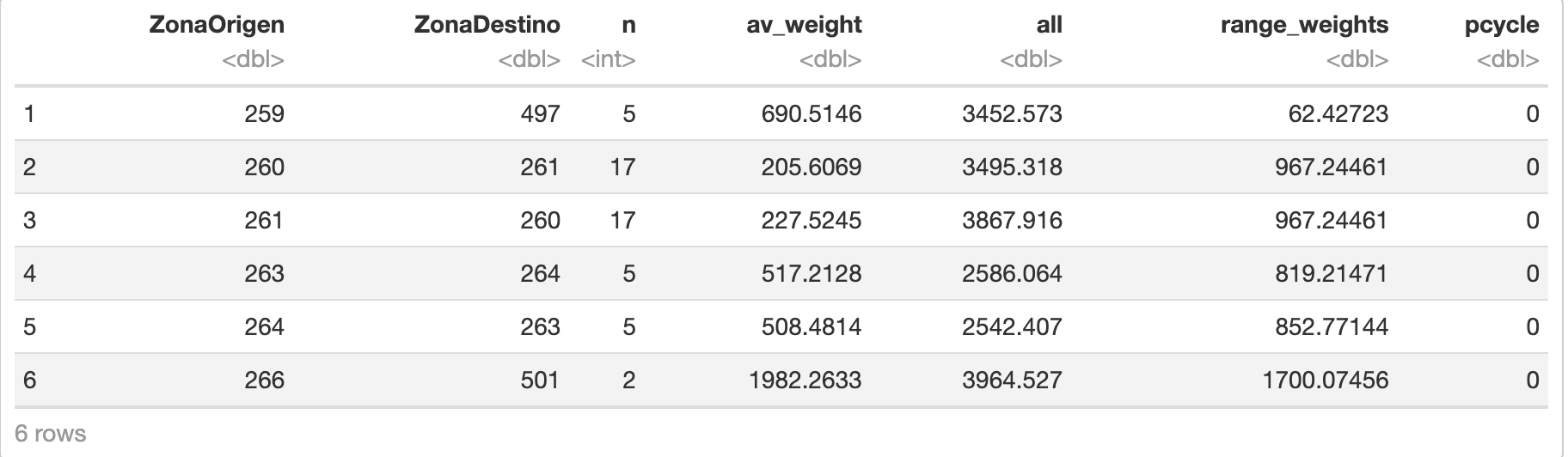
In terms of regional data, they are as follows:
sf:::print.sf(santiago_zones)
## Simple feature collection with 75 features and 1 field
## Geometry type: POLYGON
## Dimension:     XY
## Bounding box:  xmin: -70.69203 ymin: -33.47766 xmax: -70.58239 ymax: -33.403
## Geodetic CRS:  WGS 84
## First 10 features:
##     geo_code                       geometry
## 259      259 POLYGON ((-70.65174 -33.431...
## 260      260 POLYGON ((-70.65008 -33.443...
## 261      261 POLYGON ((-70.64562 -33.437...
## 262      262 POLYGON ((-70.64643 -33.477...
## 263      263 POLYGON ((-70.64913 -33.459...
## 264      264 POLYGON ((-70.64914 -33.459...
## 265      265 POLYGON ((-70.65058 -33.450...
## 266      266 POLYGON ((-70.65058 -33.450...
## 292      292 POLYGON ((-70.60615 -33.419...
## 293      293 POLYGON ((-70.60673 -33.415...
plot(santiago_zones)

Note that we have circular estimates for each desire line.
If this data is unknown, the current riding level of all desire line s can be approximated to the city's average level, such as about 5% in Santiago.
3. Create desired lines
You can use the following methods to convert the start-end data into a geographic path through the function od2line of stplanr:
desire_lines = stplanr::od2line(flow = santiago_od, zones = santiago_zones)
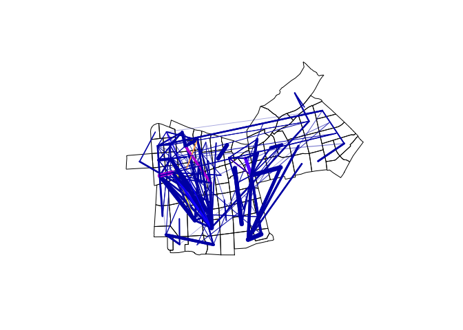
You can then draw the result line at the top of the area data as follows:
plot(santiago_zones$geometry)
plot(santiago_lines["pcycle"], lwd = santiago_lines$n / 3, add = TRUE)
# gj = geojsonsf::sf_geojson(santiago_lines)
# path = file.path(tempdir(), "dl.geojson")
# write(gj, path)
# html_map = geoplumber::gp_map(path, browse_map = FALSE)
# htmltools::includeHTML(html_map)
Previous maps show that the data are reliable: we have created a good approximation of the travel patterns in downtown San Diego.
4. Estimated bicycle usage
In order to estimate the riding potential, we need to estimate the distance and hills.
The surveyed area is relatively flat, so we can simplify the assumption that the hills of all lines are 0% (we usually get this information from the road network information):
desire_lines$hilliness = 0
What about the distance?
We can calculate it as follows (note that we convert it to a digital object to prevent problems associated with the units package):
desire_lines$distance = as.numeric(sf::st_length(desire_lines))
Now that we have a (very) rough estimate of the distance and hills, we can estimate the riding potential as follows:
desire_lines$godutch_pcycle = uptake_pct_godutch(distance = desire_lines$distance, gradient = 0)
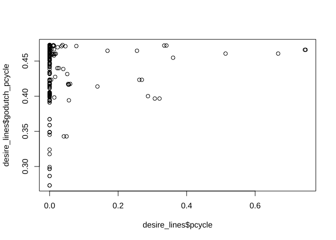
Let's look at the results, compared with the current riding level and compared with the distance:
cor(x = desire_lines$pcycle, y = desire_lines$godutch_pcycle)
## [1] 0.08743354
plot(x = desire_lines$pcycle, y = desire_lines$godutch_pcycle)
plot(x = desire_lines$distance, y = desire_lines$godutch_pcycle, ylim = c(0, 1))

As expected, there is a positive (albeit small) correlation between current and potential cycle levels.
The results clearly show that the distance attenuation begins after 2 km, but there is still a 25% share at 8 km, indicating the main shift to cycling.
We can put the results on the map as follows:
library(leaflet)
leaflet(width = "100%") %>%
  addTiles() %>%
  addPolylines(data = desire_lines, weight = desire_lines$pcycle * 5)
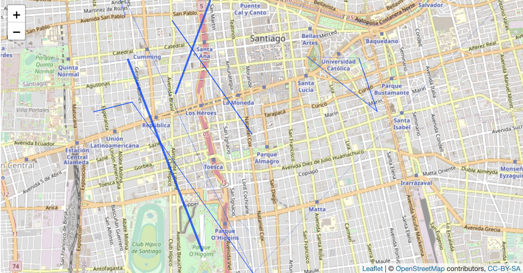
leaflet(width = "100%")
 %>% addTiles()
 %>% addPolylines(data = desire_lines, weight = desire_lines$godutch_pcycle * 5)
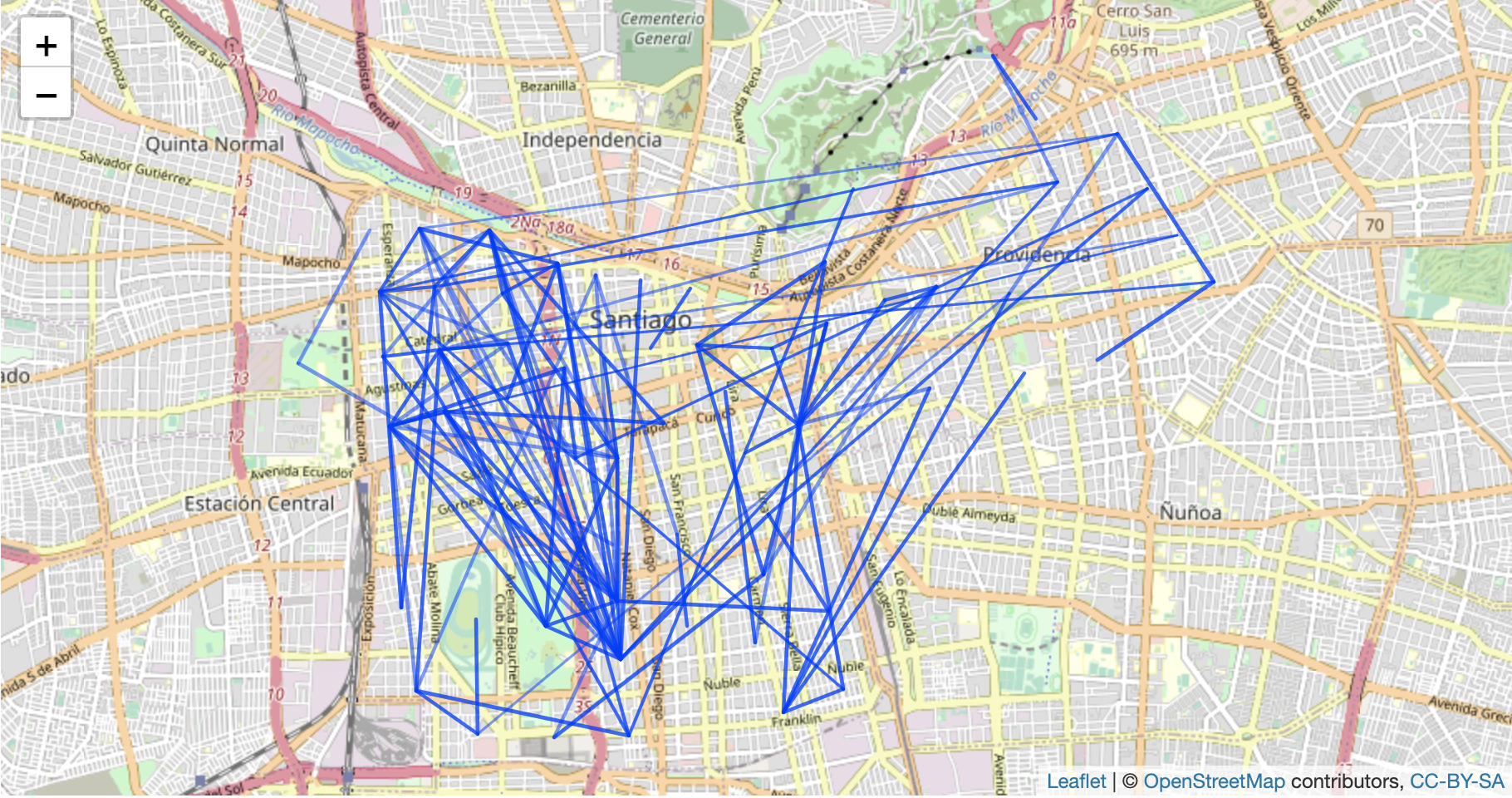
The results show that according to OD data alone, the bicycle riding level in central Santiago has great potential to improve.
However, to inform policy, more detailed estimates of bicycle potential are needed, and the results go deep into the level of each street.
This involves the road network.
5. Path
There are many ways to calculate the path on the street network.
The primary option is local routing, where the calculation is based on locally stored data (on your computer) and road network services, where the data is done remotely ("in the cloud").
Let's use the remote routing service to convert the straight line generated in the previous section into a route that people can actually ride
leaflet() %>%
  addTiles() %>%
  addPolylines(data = santiago_routes_cs[32, ])
The results show that one end of the route is connected to Sendero Ciclistas that the routing service may not be able to reach.
There are two main options at this stage:
- 1. Omit data points from the analysis and admit that the data is incomplete or incomplete
- 2. Determine the nearby location to which the service can be routed.
In this case, we will use option 1.
Before we delete the problematic line 32 from the analysis, we will connect the data from the expected line back to the result:
routes = sf::st_sf(
  cbind(sf::st_drop_geometry(santiago_routes_cs),
  sf::st_drop_geometry(desire_lines)),
  geometry = santiago_routes_cs$geometry
)
Update results
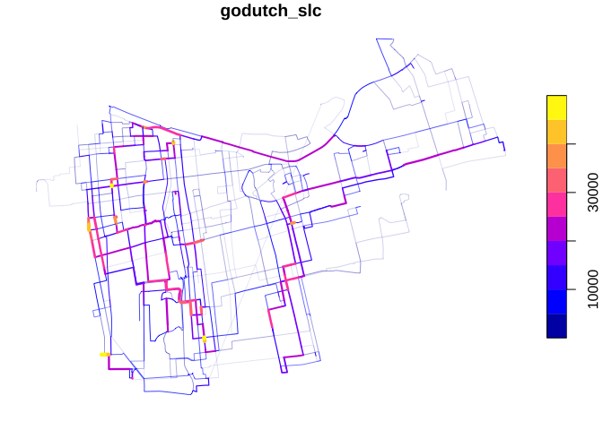
routes$godutch_slc = round(routes$godutch_pcycle * routes$all)
rnet = stplanr::overline2(routes, "godutch_slc")
plot(rnet, lwd = rnet$godutch_slc / mean(rnet$godutch_slc))
5. Further
If you are interested in this research direction / data set / processing method, you can further learn the following materials: