Preliminary exploration of Opencv source code
preface
This blog is mainly to record some learning experiences about opencv library, and intersperse some basic knowledge of image processing.
The analysis is based on opencv 4.5.1. There may be some interface changes in other versions. Please also note.
prepare
The first is the installation of opencv. For the python version of opencv, you can directly use pip install to install it. For the C + + version, you can download the source code for compilation and installation. Here is how to compile the source code under ubuntu:
tool: git,cmake
First, you need to download the source code (open source):
https://github.com/opencv/opencv
Because git may be slow, instructions such as wget/curl can be used under linux or mac to download by proxy to speed up the download speed. You can also go to the online disk I share:
Link: https://pan.baidu.com/s/1ZKOH1ehXm3gmU749lwZRlw
Extraction code: 0 wov
The second is configuration. The configuration of opencv requires cmake.
mkdir build && cd build // New build folder for building
cmake .. // Generate makefile file
make && make install // Compile and install
Note: compilation options can be configured when cmake generates Makefile. In addition, because the project is large and the compilation time is long, you can also add -j4 and use multithreading for compilation.
When calling cmake, if the error message prompts that you need to create another file to store the compiled products, you can try cmakecache Txt delete.
After installation, you can use a simple demo to test.
C++:
#include <opencv2/opencv.hpp>
using namespace cv;
int main(int argc, char **argv) {
    ///Pass the path of the file into opencv for reading
    Mat a = imread(argv[1]);
    imshow("test", a);
    waitKey(0);
    return 0;
}
CMakefile:
cmake_minimum_required(VERSION 2.8)
project( LearnOpenCV ) # The name of the file can be given casually, which corresponds to the following
find_package( OpenCV REQUIRED )
include_directories ( ${OpenCV_INCLUDE_DIRS} )
add_executable( LearnOpenCV test.cpp ) # The input file name should also correspond to
target_link_libraries( LearnOpenCV ${OpenCV_LIBS} )
Finally, use CMake and make to compile. Find a picture to test. If it can be displayed normally, it should be no problem. Of course, you can also use g++/clang + + to compile directly, but you need to pay attention to adding the binary file of opencv when linking.
Arch
The project file structure of opencv is also divided according to modules, and the source files are basically placed in the modules folder. Among them, several important modules are as follows:
1. core contains some basic class definitions, such as matrix class Mat, mask and blend operations
2. imgproc, which contains a large number of image processing algorithms, is also the focus of this blog
3. highgui, imgcodecs, videoio, including image / video codec and other functions
4. feature2d, including APIs related to 2d image feature detection
5. calib3d, 3d camera related Library
For each module, the basic file structure is as follows:
1. doc contains module related documents
2. include contains the header file (. hpp) of the module
3. misc contains some source files of other languages, including python, java, oc, etc
4. perf contains performance test related files
5. src module source file
6. Test contains unit test related files
Read / Write / Show
Images are often read before using them. The api is as follows:
Mat imread( const String& filename, int flags = IMREAD_COLOR );
The corresponding is implemented in loadsave.com in imgcodecs module Cpp file. Do some checks and initialize a Mat container, then call the imread_ in the same file. Function. The simplified steps are as follows:
static bool
imread_( const String& filename, int flags, Mat& mat )
{
    ImageDecoder decoder;
    decoder = findDecoder( filename ); ///Find a suitable decoder to parse the file
    if( !decoder ){ ///Return if not found
        return 0;
    }

    int scale_denom = 1;
    ...
    decoder->setScale( scale_denom ); ///Set scale
    decoder->setSource( filename ); ///Set source file name
    ...
    ///Make sure the file size of decode is not too large
    Size size = validateInputImageSize(Size(decoder->width(), decoder->height()));
    ///Gets the type of the picture corresponding to the decoder
    int type = decoder->type();
    type = ...
    ///Create a matrix of size height * width and type
    mat.create( size.height, size.width, type );
    ///Read picture data
    bool success = false;
    try
    {
        if (decoder->readData(mat))
            success = true;
    }
    catch ...
    if (!success)
    {
        mat.release();
        return false;
    }
    ...
    return true;
}
After such a step, the picture will call the image decoder that can decode the corresponding type according to the specific type, and readData will read the file into the matrix. Finally, it returns true, indicating that the reading is successful. The reading methods of each type of image are different, but they will eventually be transformed into a matrix (usually BGR or grayscale image), and the subsequent processing is aimed at the matrix.
The write operation is similar. First, search to find a suitable image encoder, then pass in the type, set the destination file name, and then transfer the specific write logic to the encoder.
imshow is located in the window of highgui module CPP. The definition is shown in the following code:
void cv::imshow( const String& winname, InputArray _img )
{
    CV_TRACE_FUNCTION();
    const Size size = _img.size();
#ifndef HAVE_OPENGL
    /// show with cvShowImage
#else
    const double useGl = getWindowProperty(winname, WND_PROP_OPENGL);
    CV_Assert(size.width>0 && size.height>0);
    if (useGl <= 0)
    {
        /// show with cvShowImage
    }
    else
    {
        ...
        setOpenGlContext(winname);
        cv::ogl::Texture2D& tex = ownWndTexs[winname];
        /// copy buffer from image to texture
        if (_img.kind() == _InputArray::CUDA_GPU_MAT)
        {
            cv::ogl::Buffer& buf = ownWndBufs[winname];
            buf.copyFrom(_img);
            buf.setAutoRelease(false);

            tex.copyFrom(buf);
            tex.setAutoRelease(false);
        }
        else
        {
            tex.copyFrom(_img);
        }
        setOpenGlDrawCallback(winname, glDrawTextureCallback, &tex);
        updateWindow(winname);
    }
#endif
}
There are two branch lines in the logic of drawing. If OpenGL can be used, it is preferred to use opengl for drawing (OpenGL is not used by default at present). If OpenGL is not supported, opencv also provides drawing APIs such as gtk, qt, w32 and winrt. Several cvupdatewindow and setopengldrawcallback functions in the namespace cv are empty. If the corresponding library is selected in the configuration, add the compilation. In this way, the implementation mode of drawing can be configured dynamically.
Dip
The knowledge involved in image processing is very complex, so only filter, canny and morphology are selected here to analyze how the source code is implemented.
Filter
Filtering is a core step in image processing. The C + + layer interface is as follows:
CV_EXPORTS_W void filter2D( InputArray src, OutputArray dst, int ddepth,
                            InputArray kernel, Point anchor = Point(-1,-1),
                            double delta = 0, int borderType = BORDER_DEFAULT );
filter2D in opencv is not convolution in the mathematical sense, but correlation. The convolution in mathematics needs to flip the kernel first. If the kernel range exceeds the image, the image is interpolated using the given border mode. After numerical extraction, the function is implemented as follows (in the filter.dispatch.cpp file of imgproc module):
bool res;
res = replacementFilter2D(...);
if (res)
    return;
res = dftFilter2D(...);
if (res)
    return;
ocvFilter2D(...);
It can be seen that there are three branches in the processing of filter function. The first is replacementFilter2D, which uses ipp(Integrated Performance Primitives, including a set of high-speed algorithms implemented in hardware). If the second method based on DFT (inverse Fourier transform) is not supported. When there is no other way to calculate, the most feasible way can be adopted.
ocvFilter2D
In ocvFilter2D, the createLinearFilter function is called to create a FilterEngine.
static void ocvFilter2D(...) {
    ...
    Ptr<FilterEngine> f = createLinearFilter(...);
    f->apply(...);
}
In createLinearFilter, getLinearFilter function is called to obtain the linear filter, and then it is wrapped in FilterEngine. getLinearFilter finally uses filter simd. The template class Filter2D in HPP.
The apply function is called to FilterEngine__. Apply function. First, use FilterEngine__start initializes and checks, then calls FilterEngine__. Proceed finally calls the Filter2D operator() to implement the filtering (essentially two for loops).
dftFilter2D
The filter using dft version is as follows: firstly, the size of the largest core will be determined according to whether the hardware supports it and the types of original matrix and target matrix. If the kernel is very small, false is returned, which means that dft mode is not adopted. Finally, linear filtering will be used. dft is usually used when the core is greater than 11 x 11.
After a conditional check, a new temp matrix is created, then crossCorr is called for computation, and finally the temp matrix is copied to dst, and then the success information is returned.
static bool dftFilter2D(...)
{
    {
        ...
        int dft_filter_size = ... ? 130 : 50;
        if (kernel_width * kernel_height < dft_filter_size)
            return false;
        ...
    }
    ...
    // crossCorr doesn't accept non-zero delta with multiple channels
    if (src_channels != 1 && delta != 0) {
        create Mat temp
        crossCorr(src, kernel, temp, anchor, 0, borderType);
        add(temp, delta, temp);
        ...
    } else {
        create Mat tmp
        crossCorr(src, kernel, temp, anchor, delta, borderType);
        ...
    }
    return true;
}
The crossCorr function is implemented in templmatch of imgproc module Cpp file. The basic idea is to calculate an appropriate matrix size after dft, dft the original image and core respectively, then multiply them in the frequency domain space (call the mulspectra function), and finally restore to the original size using idft. The most complex point is the determination of the size of the matrix: too small will lead to the loss of accuracy, and too large will increase the computational complexity. The most suitable size in opencv is hardcode:
// Enumerate all the best sizes within 2 ^ 32, and finally use binary search to calculate the most appropriate size
static const int optimalDFTSizeTab[] = {
    1, 2, 3, 4, 5, 6, 8, 9, 10, 12, 15, 16, ...}
Medium Filter
Median filtering is also common in image processing. It realizes the mediun in imgproc module_ blur. dispatch. Cpp file.
void medianBlur( InputArray _src0, OutputArray _dst, int ksize )
{
    ...
    // 1. Give priority to opencl. If the result can be calculated successfully, it will be returned directly
    CV_OCL_RUN(_dst.isUMat(),
               ocl_medianFilter(_src0,_dst, ksize))

    Mat src0 = _src0.getMat();
    _dst.create( src0.size(), src0.type() );
    Mat dst = _dst.getMat();
    // 2. Try cv_hal_medianBlur function performs median filtering. In the current version, this function is empty by default.
    // Here should be reserved for the entry of self-made median filter function
    CALL_HAL(medianBlur, cv_hal_medianBlur, src0.data, src0.step, dst.data, dst.step, src0.cols, src0.rows, src0.depth(),
             src0.channels(), ksize);
    // 3. Try to use openvx for median filtering
    CV_OVX_RUN(true,
               openvx_medianFilter(_src0, _dst, ksize))
    // 4. Finally, use medianblur simd. Calculation of median filter by HPP
    CV_CPU_DISPATCH(medianBlur, (src0, dst, ksize),
        CV_CPU_DISPATCH_MODES_ALL);
}
For further analysis, enter medianblur simd. Check the implementation of opencv built-in median filter in HPP file.
void medianBlur(const Mat& src0, /*const*/ Mat& dst, int ksize) {
    ...
    bool useSortNet = ...;
    Mat src;
    if ( useSortNet ) {
        ...
        if( src.depth() == CV_8U )
            medianBlur_SortNet<MinMax8u, MinMaxVec8u>( src, dst, ksize );
        else if( src.depth() == CV_16U )
            medianBlur_SortNet<MinMax16u, MinMaxVec16u>( src, dst, ksize );
        else if( src.depth() == CV_16S )
            medianBlur_SortNet<MinMax16s, MinMaxVec16s>( src, dst, ksize );
        else if( src.depth() == CV_32F )
            medianBlur_SortNet<MinMax32f, MinMaxVec32f>( src, dst, ksize );
        else
            CV_Error(CV_StsUnsupportedFormat, "");
        return;
    } else {
        ///Create border
        cv::copyMakeBorder( src0, src, 0, 0, ksize/2, ksize/2, BORDER_REPLICATE|BORDER_ISOLATED);
        if( ksize <= ...) medianBlur_8u_Om( src, dst, ksize );
        else medianBlur_8u_O1( src, dst, ksize );
    }
}
It can be seen that there are three outlets for median filtering. First, judge whether to use SortNet according to the size of the core (3 or 5). If yes, enter medianBlur_SortNet method. Then judge again according to the size of the core. If the core is relatively small, use a general Om median filter. If the core is relatively large, use an O1 median filter.
Now go to medianBlur_SortNet method to view the implementation. It can be seen that only the median filtering in the case of m = 3 and m = 5 is processed here. At the same time, this method is a generic method, which passes in Op and VecOp, which correspond to the size comparison between two values and the size comparison between two vectors respectively.
template<class Op, class VecOp>
static void
medianBlur_SortNet( const Mat& _src, Mat& _dst, int m )
{
    CV_INSTRUMENT_REGION();

    typedef typename Op::value_type T;
    typedef typename Op::arg_type WT;
    typedef typename VecOp::arg_type VT;

    const T* src = _src.ptr<T>();
    T* dst = _dst.ptr<T>();
    int sstep = (int)(_src.step/sizeof(T));
    int dstep = (int)(_dst.step/sizeof(T));
    Size size = _dst.size();
    int i, j, k, cn = _src.channels();
    Op op;
    VecOp vop;

    if( m == 3 ) {
        if( size.width == 1 || size.height == 1 ) {
            ///Dealing with extreme situations
            return;
        }
        size.width *= cn;
        ///Traverse each line
        for( i = 0; i < size.height; i++, dst += dstep ) {
            const T* row0 = src + std::max(i - 1, 0)*sstep;
            const T* row1 = src + i*sstep;
            const T* row2 = src + std::min(i + 1, size.height-1)*sstep;
            int limit = cn;
            ///Traverse each column
            for(j = 0;; ) {
                ///Traverse cn pixels and compare each channel to get the median value
                for( ; j < limit; j++ )
                {
                    int j0 = j >= cn ? j - cn : j;
                    int j2 = j < size.width - cn ? j + cn : j;
                    WT p0 = row0[j0], p1 = row0[j], p2 = row0[j2];
                    WT p3 = row1[j0], p4 = row1[j], p5 = row1[j2];
                    WT p6 = row2[j0], p7 = row2[j], p8 = row2[j2];
                    ///op(p1, p2) is used to exchange two numbers when P1 < P2
                    op(p1, p2); op(p4, p5); op(p7, p8); op(p0, p1);
                    op(p3, p4); op(p6, p7); op(p1, p2); op(p4, p5);
                    op(p7, p8); op(p0, p3); op(p5, p8); op(p4, p7);
                    op(p3, p6); op(p1, p4); op(p2, p5); op(p4, p7);
                    op(p4, p2); op(p6, p4); op(p4, p2);
                    dst[j] = (T)p4;
                }

                if( limit == size.width )
                    break;

                for( ; j <= size.width - VecOp::SIZE - cn; j += VecOp::SIZE )
                {
                    VT p0 = vop.load(row0+j-cn), p1 = vop.load(row0+j), p2 = vop.load(row0+j+cn);
                    VT p3 = vop.load(row1+j-cn), p4 = vop.load(row1+j), p5 = vop.load(row1+j+cn);
                    VT p6 = vop.load(row2+j-cn), p7 = vop.load(row2+j), p8 = vop.load(row2+j+cn);

                    vop(p1, p2); vop(p4, p5); vop(p7, p8); vop(p0, p1);
                    vop(p3, p4); vop(p6, p7); vop(p1, p2); vop(p4, p5);
                    vop(p7, p8); vop(p0, p3); vop(p5, p8); vop(p4, p7);
                    vop(p3, p6); vop(p1, p4); vop(p2, p5); vop(p4, p7);
                    vop(p4, p2); vop(p6, p4); vop(p4, p2);
                    vop.store(dst+j, p4);
                }
                limit = size.width;
            }
        }
    }
    else if( m == 5 ) {
        ///Similar to the processing method of m == 3 above, use as few comparisons as possible to get the median value
    }
}
The implementation of Op is MinMax in the same file? Class,? 8u, 16U, 16S and 32F respectively. The specific operation is to exchange these two numbers when the first parameter is larger than the first parameter. Note that the operator() method in the corresponding class of MinMax8u is somewhat different:
int t = CV_FAST_CAST_8U(a - b);
b += t; a -= t;
Also, if CVS are not enabled_ SIMD (simple instruction multiple data), VecOp and Op are equivalent. A major optimization of this method is that it uses loop expansion and multiple MinMax operations to obtain the median instead of loop traversal, which speeds up the execution speed of the code.
Another method to realize median filtering is medianblur_ 8u_ The implementation of OM is completely different. An interesting point is that it calculates the median by directly counting the occurrence times of 0 ~ 255 pixels in the matrix covered by the kernel. Then, as long as the number of occurrences of a certain x is greater than half the size of the core, X is filled in the result matrix. The problem caused by this is that in the worst case, 256 values need to be traversed at a time, so a simple optimization is adopted in the algorithm: interval statistics. A new array of size 16 is used to represent the occurrence times of [0... 15], [16... 31]... Respectively. In this way, the speed of finding the median point is much faster. In the worst case, you only need to traverse 32 values to get the median point.
Canny
Canny algorithm is a classic edge extraction algorithm. The imgproc module of opencv has a separate canny Cpp file is responsible for completing Canny algorithm. The entry function is as follows:
///src is the input matrix and dst is the output matrix
/// low_thresh and high_thresh is the high and low threshold respectively
/// aperture_size is the Sobel aperture size (3, 5 or 7)
///L2Gradient indicates whether to use L2 gradient
void Canny( InputArray _src, OutputArray _dst,
                double low_thresh, double high_thresh,
                int aperture_size, bool L2gradient )
{
    ///Some basic condition checks
    const Size size = _src.size();
    ...
    ///The openipl algorithm will be used to complete the calculation, and the openipl algorithm will be used to directly complete the calculation
    CV_OCL_RUN(...)
    CALL_HAL(...);
    CV_OVX_RUN(...)
    CV_IPP_RUN_FAST(...)
    ///When using l2radio, the thresh needs to be corrected
    if (L2gradient)
    {
        low_thresh = std::min(32767.0, low_thresh);
        high_thresh = std::min(32767.0, high_thresh);
        if (low_thresh > 0) low_thresh *= low_thresh;
        if (high_thresh > 0) high_thresh *= high_thresh;
    }
    int low = cvFloor(low_thresh);
    int high = cvFloor(high_thresh);
    ///Calculate how many threads are used to calculate canny according to the number of threads running in opencv and the number of cpu cores
    int numOfThreads = ...;

    Mat map;
    std::deque<uchar*> stack;
    ///Parallel computing canny
    parallel_for_(Range(0, src.rows), parallelCanny(src, map, stack, low, high, aperture_size, L2gradient), numOfThreads);
    ///Perform global edge track in turn
    ptrdiff_t mapstep = map.cols;
    while (!stack.empty())
    {
        uchar* m = stack.back();
        stack.pop_back();

        if (!m[-mapstep-1]) CANNY_PUSH((m-mapstep-1), stack);
        if (!m[-mapstep])   CANNY_PUSH((m-mapstep), stack);
        if (!m[-mapstep+1]) CANNY_PUSH((m-mapstep+1), stack);
        if (!m[-1])         CANNY_PUSH((m-1), stack);
        if (!m[1])          CANNY_PUSH((m+1), stack);
        if (!m[mapstep-1])  CANNY_PUSH((m+mapstep-1), stack);
        if (!m[mapstep])    CANNY_PUSH((m+mapstep), stack);
        if (!m[mapstep+1])  CANNY_PUSH((m+mapstep+1), stack);
    }
    ///Finally, go through the map and turn the points marked edge in the map into 255 and the other points into 0
    parallel_for_(Range(0, src.rows), finalPass(map, dst), src.total()/(double)(1<<16));
}
It can be seen that the core calculation function is parallelCanny, which uses multithreading for calculation. The calculation process can be divided into the following steps (without considering SIMD, some codes will be different when considering SIMD).
sobel operator
canny's first step is to use sobel operator to calculate the gradient of each point in the x and y directions. The two function calls of the core are as follows:
if(needGradient)
{
    Sobel(src.rowRange(rowStart, rowEnd), dx, CV_16S, 1, 0, aperture_size, scale, 0, BORDER_REPLICATE);
    Sobel(src.rowRange(rowStart, rowEnd), dy, CV_16S, 0, 1, aperture_size, scale, 0, BORDER_REPLICATE);
}
According to the given parameters, the core of sobel involved in the calculation is:
kernelX = [[-1, 0, 1]]
kernelY = [[-1],[0],[1]]
The calculated results are stored in dx and dy matrices.
Edge detect
In order to make better use of space, a circular buffer is used here to save the intensity of each point in each line of the image. mag_a represents the current line, mag_p stands for the previous line, mag_n indicates the next line.
AutoBuffer<int> buffer(3 * (mapstep * cn));
_mag_p = buffer.data() + 1;
_mag_a = _mag_p + mapstep * cn;
_mag_n = _mag_a + mapstep * cn;
Next, traverse each line of the thread and calculate the size of the magnet. Then, non maximum suppression is carried out to obtain the relevant information of whether each point belongs to edge. Expressed by matrix pmap, each point 2 indicates that the point is an edge, 1 indicates that the point cannot be an edge, and 0 indicates that the point may be an edge.
///rowStart and end respectively represent the rows of the image that the current thread is responsible for
for (int i = rowStart; i <= boundaries.end; ++i) {
    /*  Calculate the magnitude part  */
    ///Calculate the magnitude of the next line
    if(i < rowEnd) {
        _dx = dx.ptr<short>(i - rowStart);
        _dy = dy.ptr<short>(i - rowStart);
        ///Calculate gradient using L2
        if (L2gradient)
        {
            int j = 0, width = src.cols * cn;
            for ( ; j < width; ++j)
                _mag_n[j] = int(_dx[j])*_dx[j] + int(_dy[j])*_dy[j];
        } else { ///Calculate gradient using L1
            int j = 0, width = src.cols * cn;
            for ( ; j < width; ++j)
                _mag_n[j] = std::abs(int(_dx[j])) + std::abs(int(_dy[j]));
        }
        ...
    } else {
        ...
    }
    ...
    /*  Non maximum suppression part  */
    ///The size of tan22 is 13573 / (1 < < 16), and the accuracy is improved by integer
    const int TG22 = 13573;
    int j = 0;
    for (; j < src.cols; j++) {
        int m = _mag_a[j];
        if (m > low) {
            short xs = _dx[j];
            short ys = _dy[j];
            int x = (int)std::abs(xs);
            int y = (int)std::abs(ys) << 15;

            int tg22x = x * TG22;
            ///The gradient is horizontal
            if (y < tg22x)
            {
                if (m > _mag_a[j - 1] && m >= _mag_a[j + 1])
                {
                    ///Judge whether the gradient of the point is greater than the threshold high. If so, push it into the stack, and pmap is set to 0
                    ///Similar below
                    CANNY_CHECK(m, high, (_pmap+j), stack);
                    continue;
                }
            }
            else
            {
                ///The gradient is in the vertical direction
                int tg67x = tg22x + (x << 16);
                if (y > tg67x)
                {
                    if (m > _mag_p[j] && m >= _mag_n[j])
                    {
                        CANNY_CHECK(m, high, (_pmap+j), stack);
                        continue;
                    }
                }
                else
                {
                    ///The gradient is in the oblique direction
                    int s = (xs ^ ys) < 0 ? -1 : 1;
                    if(m > _mag_p[j - s] && m > _mag_n[j + s])
                    {
                        CANNY_CHECK(m, high, (_pmap+j), stack);
                        continue;
                    }
                }
            }
        }
        _pmap[j] = 1;
    }
}
Edge track
In the previous function, we have calculated the information that pmap indicates whether each node can be an edge. The double threshold algorithm requires that the nodes that may be edges can be counted as edges only if there are certain edge nodes in the surrounding eight points, otherwise the current point does not belong to edges. Therefore, the algorithm uses a data structure such as stack to implement. All nodes that must be edges are put into the stack. When processing each node, the surrounding eight nodes, if there are nodes that may be edges, are marked as edges and incorporated into the stack until the stack is empty.
while (!stack.empty())
{
    uchar *m = stack.back();
    stack.pop_back();
    if(/* Not at boundary */ (unsigned)(m - pmapLower) < pmapDiff) {
        if (!m[-mapstep-1]) CANNY_PUSH((m-mapstep-1), stack);
        if (!m[-mapstep])   CANNY_PUSH((m-mapstep), stack);
        if (!m[-mapstep+1]) CANNY_PUSH((m-mapstep+1), stack);
        if (!m[-1])         CANNY_PUSH((m-1), stack);
        if (!m[1])          CANNY_PUSH((m+1), stack);
        if (!m[mapstep-1])  CANNY_PUSH((m+mapstep-1), stack);
        if (!m[mapstep])    CANNY_PUSH((m+mapstep), stack);
        if (!m[mapstep+1])  CANNY_PUSH((m+mapstep+1), stack);
    } else {
        ///Handling boundary conditions
    }
}
After the above steps, there may be some problems on the boundary because the edge track operation is only carried out locally. Therefore, the canny algorithm of opencv also adds a global track operation. The code is similar to that above and will not be repeated.
Final pass
The last step is to map the point marked 2 in pmap to 255, and 0 or 1 to 0. The code is as follows:
// the final pass, form the final image
for (int i = boundaries.start; i < boundaries.end; i++)
{
    int j = 0;
    uchar *pdst = dst.ptr<uchar>(i);
    const uchar *pmap = map.ptr<uchar>(i + 1);
    pmap += 1;
    for (; j < dst.cols; j++)
    {
        pdst[j] = (uchar)-(pmap[j] >> 1);
    }
}
Note that pmap+1 in the code is because pmap adds a boundary with a width of 1 to the original image.
Uchar means 0 of uchar type. After PMAP [J] > > 1, it is 1 only when pmap[j] = 2. Therefore, 2 is mapped to 255 (white) and 0 / 1 is mapped to 0 (black), that is, the image after boundary extraction is obtained.
Morph
morph.dispatch.cpp class provides a method to construct the kernel of morphological operation, as follows:
Mat getStructuringElement(int shape, Size ksize, Point anchor)
{
    int i, j;
    int r = 0, c = 0;
    double inv_r2 = 0;

    anchor = normalizeAnchor(anchor, ksize);
    if( ksize == Size(1,1) )
        shape = MORPH_RECT;
    if( shape == MORPH_ELLIPSE )
    {
        r = ksize.height/2;
        c = ksize.width/2;
        inv_r2 = r ? 1./((double)r*r) : 0;
    }

    Mat elem(ksize, CV_8U);
    for( i = 0; i < ksize.height; i++ )
    {
        uchar* ptr = elem.ptr(i);
        int j1 = 0, j2 = 0;
        ///When the shape is a rectangle or a cross is just on the horizontal line, fill a whole line directly
        if( shape == MORPH_RECT || (shape == MORPH_CROSS && i == anchor.y) )
            j2 = ksize.width;
        else if( shape == MORPH_CROSS )
            j1 = anchor.x, j2 = j1 + 1;
        else
        {
            int dy = i - r;
            if( std::abs(dy) <= r )
            {
                ///Calculate the approximate width of the ellipse
                int dx = saturate_cast<int>(c*std::sqrt((r*r - dy*dy)*inv_r2));
                j1 = std::max( c - dx, 0 );
                j2 = std::min( c + dx + 1, ksize.width );
            }
        }
        ///Fill in the numbers in the j1 ~ j2 interval
        for( j = 0; j < j1; j++ )
            ptr[j] = 0;
        for( ; j < j2; j++ )
            ptr[j] = 1;
        for( ; j < ksize.width; j++ )
            ptr[j] = 0;
    }

    return elem;
}
It can be seen that there are three shapes of nuclei, corresponding to the following:
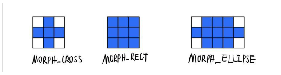
Note that the above figure is centered on the midpoint (Anchor), and can also be operated centered on other points (equivalent to offsetting the image).
In addition, various morphological operations are basically transformed into erode and dilate operations. Several common morphological operations are as follows (in the morphologyEx method in morph.dispatch.cpp file):
switch( op )
{
case MORPH_ERODE: ///Corrosion operation
    erode( src, dst, kernel, anchor, iterations, borderType, borderValue );
    break;
case MORPH_DILATE: ///Expansion operation
    dilate( src, dst, kernel, anchor, iterations, borderType, borderValue );
    break;
case MORPH_OPEN: ///On operation
    erode( src, dst, kernel, anchor, iterations, borderType, borderValue );
    dilate( dst, dst, kernel, anchor, iterations, borderType, borderValue );
    break;
case MORPH_CLOSE: ///Closed operation
    dilate( src, dst, kernel, anchor, iterations, borderType, borderValue );
    erode( dst, dst, kernel, anchor, iterations, borderType, borderValue );
    break;
case MORPH_GRADIENT: ///Gradient calculation operation
    erode( src, temp, kernel, anchor, iterations, borderType, borderValue );
    dilate( src, dst, kernel, anchor, iterations, borderType, borderValue );
    dst -= temp;
    break;
case MORPH_TOPHAT: ///Top hat operation
    if( src.data != dst.data )
        temp = dst;
    erode( src, temp, kernel, anchor, iterations, borderType, borderValue );
    dilate( temp, temp, kernel, anchor, iterations, borderType, borderValue );
    dst = src - temp;
    break;
case MORPH_BLACKHAT: ///Black hat operation
    if( src.data != dst.data )
        temp = dst;
    dilate( src, temp, kernel, anchor, iterations, borderType, borderValue );
    erode( temp, temp, kernel, anchor, iterations, borderType, borderValue );
    dst = temp - src;
    break;
...
}
The morphOp method is used for dilate and erode operations. Then call the morph method. An empty CV is provided in this method_ hal_ Morph method allows users to define the implementation of morph method. If there is no self-defined implementation, call the ocvMorph method provided by opencv. Similar to other filters, in this method, createMorphologyFilter is called to get a FilterEngine, and finally the apply method is called to calculate. Finally, a template class such as MorphFilter actually performs graphics filtering operations:
template<class Op, class VecOp> struct MorphFilter : BaseFilter
{
    typedef typename Op::rtype T;
    MorphFilter( const Mat& _kernel, Point _anchor ) { ... }

    void operator()(const uchar** src, uchar* dst, int dststep, int count, int width, int cn) CV_OVERRIDE
    {
        ...
        width *= cn;
        ///Traverse each line
        for( ; count > 0; count--, dst += dststep, src++ )
        {
            ...
            ///Traverse each column
            for( ; i < width; i++ )
            {
                T s0 = kp[0][i];
                ///Filtering operation
                for( k = 1; k < nz; k++ )
                    s0 = op(s0, kp[k][i]);
                D[i] = s0;
            }
        }
    }
};
For erode and dilate operations, you only need to pass in MinOp (the one with smaller return value) and maxop (the one with larger return value) respectively. Take erode as an example. After inputting MinOp, for each point on the core with 1, the corresponding position covered on the image must also be 1. Otherwise, due to the characteristics of min operation, as long as one point is 0, the final result will be 0. The result of this operation is that placing the core center on any point with 1 on the result image can be wrapped by the original image, That is, the resulting image is the corrosion of the source image. The expansion uses the maximum value, which is similar to the analysis.
Python extension
opencv code is written in C + +, but it also provides Python library. How do you do this? This is the extension of Python. The official documentation provides a python H library for developers, which provides various APIs for C + + and python interaction, such as:
PyModule_Create  ///Create a python module
PyModule_AddObject  ///Add an object to the module
PyModule_AddIntConstant  ///Add int constant to module
PyModule_AddStringConstant  ///Add a string constant to the module
Py_DECREF ///Recycle a python object
PyObject_Call  ///Call a python function and return a pointer to the result
...
In this way, for each C + + method that needs to be exposed to python, you only need to create a wrapper method (wrapper class), and finally return the result as a python object, similar to the following code:
static PyObject *
spam_system(PyObject *self, PyObject *args)
{
    const char *command;
    int sts;

    if (!PyArg_ParseTuple(args, "s", &command))
        return NULL;
    sts = system(command);
    return PyLong_FromLong(sts);
}
Then, you need to add pyinit_ The class named XXX is used to create the module. After init import is found and python interpreter is called, python interpreter will be started_ CV2 and call this method, we just need to create a module inside this method and add methods in the module.
In opencv, the init function is located in cv2.0 under python module Cpp file:
PyObject* PyInit_cv2() {
    import_array(); // from numpy
    PyObject* m = PyModule_Create(&cv2_moduledef);
    if (!init_body(m))
        return NULL;
    return m;
}
nit_ In the body function, create each sub module in turn and pass in the function signature.
The wrapper class and wrapper method are generated by gen2.0 under python module Py and hdr_parser.py generated, these two functions will be automatically run during compilation to generate conversion code. gen2.py calls hdr_parser.py parses the header file corresponding to each module in turn according to CV_EXPORTS_W,CV_WRAP and other macros identify whether a function / class needs to generate intermediate conversion code. After the compilation is completed, the python interpreter will find the corresponding function area and execute it during operation.