Ptorch cifar10 image classification LeNet5
Here is a summary: Summary
4. Define network (LeNet5)
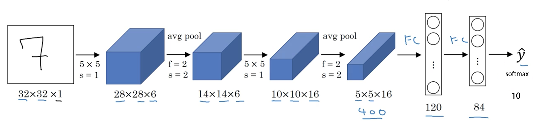
Handwritten font recognition model LeNet5 was born in 1994 and is one of the earliest convolutional neural networks. Through ingenious design, LeNet5 uses convolution, parameter sharing, pooling and other operations to extract features, avoiding a large amount of computing cost. Finally, it uses fully connected neural network for classification and recognition. This network is also the starting point of a large number of neural network architectures recently.
Some properties of LeNet-5:
-
If the input layer does not count the layers of the neural network, LeNet-5 is a 7-layer network. (convolution and pooling may also be regarded as a layer in some places) (the "5" in the name of LeNet-5 can also be understood as the number of layers with trainable parameters in the whole network is 5.)
-
LeNet-5 has approximately 60000 parameters.
-
As the network gets deeper and deeper, the height and width of the image are shrinking. At the same time, the number of channel s of the image has been increasing.
-
The current commonly used LeNet-5 structure is different from the structure proposed by Professor Yann LeCun in his 1998 paper, such as the use of activation function. Now, ReLU is generally used as the activation function, and softmax is generally selected for the output layer.
First of all, we still have to judge whether we can use GPU, because the speed of GPU may be about 20-50 times faster than that of CPU, especially for convolutional neural network.
device = 'cuda' if torch.cuda.is_available() else 'cpu'
#Define network
class LeNet5(nn.Module):# nn.Module is the base class of all neural networks. Any neural network defined by ourselves should inherit NN Module
    def __init__(self):
        super(LeNet5,self).__init__()
        self.conv1 = nn.Sequential(
            # Convolution layer 1, 3-channel input, 6 convolution kernels, kernel size 5 * 5
            # After this layer, the image size becomes 32-5 + 1, 28 * 28
            nn.Conv2d(in_channels=3,out_channels=6,kernel_size=5,stride=1, padding=0),
            #Activation function
            nn.ReLU(),
            # After 2 * 2 maximum pooling, the image becomes 14 * 14
            nn.MaxPool2d(kernel_size=2,stride=2,padding=0),
        )
        self.conv2 = nn.Sequential(
            # Convolution layer 2, 6 input channels, 16 convolution kernels, kernel size 5 * 5
            # After this layer, the image becomes 14-5 + 1, 10 * 10
            nn.Conv2d(in_channels=6,out_channels=16,kernel_size=5,stride=1, padding=0),
            nn.ReLU(),
            # After 2 * 2 maximum pooling, the image becomes 5 * 5
            nn.MaxPool2d(kernel_size=2,stride=2,padding=0),
        )
        self.fc = nn.Sequential(
            # Then there are three full connection layers
            nn.Linear(16*5*5,120),
            nn.ReLU(),
            nn.Linear(120,84),
            nn.ReLU(),
            nn.Linear(84,10),
        )

        # Define the forward propagation process, and enter
    def forward(self,x):
        x = self.conv1(x)
        x = self.conv2(x)
        # nn. The input and output of linear () are values with one dimension, so the multi-dimensional tensor should be flattened into one dimension

        x = x.view(x.size()[0],-1)
        x = self.fc(x)
        return x

net = LeNet5().cuda()
summary(net,(3,32,32))
----------------------------------------------------------------
     Layer (type)               Output Shape         Param #
================================================================
         Conv2d-1            [-1, 6, 28, 28]             456
           ReLU-2            [-1, 6, 28, 28]               0
      MaxPool2d-3            [-1, 6, 14, 14]               0
         Conv2d-4           [-1, 16, 10, 10]           2,416
           ReLU-5           [-1, 16, 10, 10]               0
      MaxPool2d-6             [-1, 16, 5, 5]               0
         Linear-7                  [-1, 120]          48,120
           ReLU-8                  [-1, 120]               0
         Linear-9                   [-1, 84]          10,164
          ReLU-10                   [-1, 84]               0
        Linear-11                   [-1, 10]             850
================================================================
Total params: 62,006
Trainable params: 62,006
Non-trainable params: 0
----------------------------------------------------------------
Input size (MB): 0.01
Forward/backward pass size (MB): 0.11
Params size (MB): 0.24
Estimated Total Size (MB): 0.36
----------------------------------------------------------------
Firstly, from our summary, we can see that the parameters of the model we defined are about 62 thousand. We input the tensor of (batch, 3, 32, 32), and here we can also see the change of our image output size after each layer. Finally, we output 10 parameters, and then we can get the probability of each category through the softmax function.
We can also print out our model and observe it
LeNet5(
  (conv1): Sequential(
    (0): Conv2d(3, 6, kernel_size=(5, 5), stride=(1, 1))
    (1): ReLU()
    (2): MaxPool2d(kernel_size=2, stride=2, padding=0, dilation=1, ceil_mode=False)
  )
  (conv2): Sequential(
    (0): Conv2d(6, 16, kernel_size=(5, 5), stride=(1, 1))
    (1): ReLU()
    (2): MaxPool2d(kernel_size=2, stride=2, padding=0, dilation=1, ceil_mode=False)
  )
  (fc): Sequential(
    (0): Linear(in_features=400, out_features=120, bias=True)
    (1): ReLU()
    (2): Linear(in_features=120, out_features=84, bias=True)
    (3): ReLU()
    (4): Linear(in_features=84, out_features=10, bias=True)
  )
)
If your computer has multiple GPUs, this code can use GPUs for parallel computing to speed up the computing speed
net =LeNet5().to(device)
if device == 'cuda':
    net = nn.DataParallel(net)
    # When the calculation diagram does not change (the shape of each input is the same, and the model does not change), the performance can be improved, otherwise, the performance will be reduced
    torch.backends.cudnn.benchmark = True
5. Define loss function and optimizer
pytorch encapsulates all the optimization methods commonly used in deep learning in torch In Optim, all optimization methods inherit the base class optim Optimizier
The loss function is encapsulated in the neural network toolbox nn, which contains many loss functions
Here I use the SGD + momentum algorithm, and our loss function is defined as the cross entropy function. In addition, the learning strategy is defined as dynamically updating the learning rate. If the training loss does not decrease after 5 iterations, we will change the learning rate, which will become 0.5 times the original, and the minimum will be reduced to 0.00001
If you want to know more about the optimizer and learning rate strategy, you can refer to the following resources
- Pytorch Note15 optimization algorithm 1 gradient descent variables
- Pytorch Note16 optimization algorithm 2 momentum method
- Ptorch note34 learning rate decay
It is decided to iterate 20 times
import torch.optim as optim
optimizer = optim.SGD(net.parameters(), lr=1e-1, momentum=0.9, weight_decay=5e-4)
criterion = nn.CrossEntropyLoss()
scheduler = optim.lr_scheduler.ReduceLROnPlateau(optimizer, 'min', factor=0.5 ,patience = 5,min_lr = 0.000001) # Dynamic update learning rate
# scheduler = optim.lr_scheduler.MultiStepLR(optimizer, milestones=[75, 150], gamma=0.5)
import time
epoch = 20
6. Training
First, define the location where the model is saved
import os
if not os.path.exists('./model'):
    os.makedirs('./model')
else:
    print('file already exist')
save_path = './model/LeNet5.pth'
I define a train function, perform a training in the train function, and save our trained model
from utils import trainfrom utils import plot_historyAcc, Loss, Lr = train(net, trainloader, testloader, epoch, optimizer, criterion, scheduler, save_path, verbose = True)
Epoch [ 1/ 20] Train Loss:1.918313 Train Acc:28.19% Test Loss:1.647650 Test Acc:39.23% Learning Rate:0.100000 Time 00:29Epoch [ 2/ 20] Train Loss:1.574629 Train Acc:42.00% Test Loss:1.521759 Test Acc:44.59% Learning Rate:0.100000 Time 00:21Epoch [ 3/ 20] Train Loss:1.476749 Train Acc:46.23% Test Loss:1.438898 Test Acc:48.56% Learning Rate:0.100000 Time 00:21Epoch [ 4/ 20] Train Loss:1.415963 Train Acc:49.10% Test Loss:1.378597 Test Acc:50.25% Learning Rate:0.100000 Time 00:21Epoch [ 5/ 20] Train Loss:1.384430 Train Acc:50.69% Test Loss:1.350369 Test Acc:51.81% Learning Rate:0.100000 Time 00:20Epoch [ 6/ 20] Train Loss:1.331118 Train Acc:52.49% Test Loss:1.384710 Test Acc:49.62% Learning Rate:0.100000 Time 00:20Epoch [ 7/ 20] Train Loss:1.323763 Train Acc:53.08% Test Loss:1.348911 Test Acc:52.59% Learning Rate:0.100000 Time 00:21Epoch [ 8/ 20] Train Loss:1.291410 Train Acc:54.19% Test Loss:1.273263 Test Acc:55.00% Learning Rate:0.100000 Time 00:20Epoch [ 9/ 20] Train Loss:1.261590 Train Acc:55.36% Test Loss:1.295092 Test Acc:54.50% Learning Rate:0.100000 Time 00:20Epoch [ 10/ 20] Train Loss:1.239585 Train Acc:56.45% Test Loss:1.349028 Test Acc:52.57% Learning Rate:0.100000 Time 00:21Epoch [ 11/ 20] Train Loss:1.225227 Train Acc:56.81% Test Loss:1.293521 Test Acc:53.87% Learning Rate:0.100000 Time 00:22Epoch [ 12/ 20] Train Loss:1.221355 Train Acc:56.86% Test Loss:1.255155 Test Acc:56.13% Learning Rate:0.100000 Time 00:21Epoch [ 13/ 20] Train Loss:1.207748 Train Acc:57.59% Test Loss:1.238375 Test Acc:57.10% Learning Rate:0.100000 Time 00:21Epoch [ 14/ 20] Train Loss:1.195587 Train Acc:58.01% Test Loss:1.185524 Test Acc:58.56% Learning Rate:0.100000 Time 00:20Epoch [ 15/ 20] Train Loss:1.183456 Train Acc:58.50% Test Loss:1.192770 Test Acc:58.04% Learning Rate:0.100000 Time 00:21Epoch [ 16/ 20] Train Loss:1.168697 Train Acc:59.13% Test Loss:1.272912 Test Acc:55.85% Learning Rate:0.100000 Time 00:20Epoch [ 17/ 20] Train Loss:1.167685 Train Acc:59.23% Test Loss:1.195087 Test Acc:58.33% Learning Rate:0.100000 Time 00:20Epoch [ 18/ 20] Train Loss:1.162324 Train Acc:59.37% Test Loss:1.242964 Test Acc:56.62% Learning Rate:0.100000 Time 00:21Epoch [ 19/ 20] Train Loss:1.154494 Train Acc:59.72% Test Loss:1.274993 Test Acc:54.90% Learning Rate:0.100000 Time 00:21Epoch [ 20/ 20] Train Loss:1.163650 Train Acc:59.45% Test Loss:1.182077 Test Acc:59.00% Learning Rate:0.100000 Time 00:20
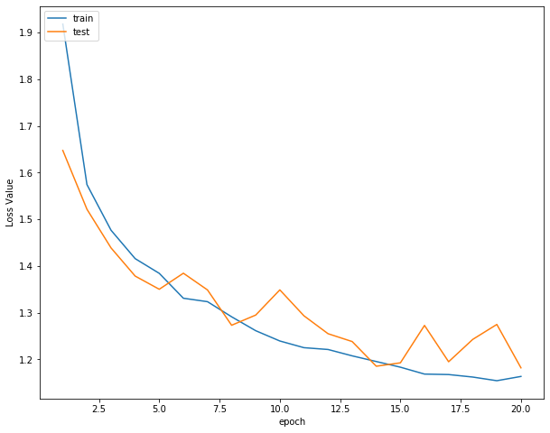
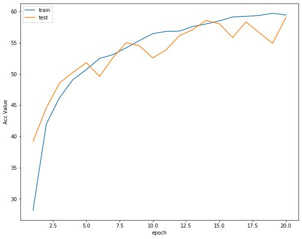
Then you can print the loss function curve, accuracy curve and learning rate curve respectively
plot_history(epoch ,Acc, Loss, Lr)
Loss function curve
Accuracy curve
Learning rate curve

7. Test
View accuracy
correct = 0   # Define the number of pictures predicted correctly and initialize to 0
total = 0     # The total number of pictures participating in the test is also initialized to 0
# testloader = torch.utils.data.DataLoader(testset, batch_size=32,shuffle=True, num_workers=2)
for data in testloader:  # Cycle each batch
    images, labels = data
    images = images.to(device)
    labels = labels.to(device)
    net.eval()  # Change the model to test mode
    if hasattr(torch.cuda, 'empty_cache'):
        torch.cuda.empty_cache()
    outputs = net(images)  # Input network for testing

    # outputs.data is a 4x10 tensor. The value and sequence number of the largest column in each row form a one-dimensional tensor. The first is the tensor of value and the second is the tensor of sequence number.
    _, predicted = torch.max(outputs.data, 1)
    total += labels.size(0)          # Update the number of test pictures
    correct += (predicted == labels).sum() # Update the number of correctly classified pictures

print('Accuracy of the network on the 10000 test images: %.2f %%' % (100 * correct / total))
Accuracy of the network on the 10000 test images: 59.31 %
It can be seen that the accuracy of the self-defined network model in the test set is 59.31%
Torch in the program Max (outputs. Data, 1), returns a tuple
It is obvious here that the first element of the returned tuple is image data, that is, the maximum value, and the second element is label, that is, the index of the maximum value! We only need label (the index of the maximum value), so there will be an assignment statement such as, predicted, which means to ignore the first return value and assign it to, which means to discard it;
Check the accuracy of each category
 # Define 2 lists that store the correct number of tests in each class, and initialize to 0
class_correct = list(0. for i in range(10))
class_total = list(0. for i in range(10))
# testloader = torch.utils.data.DataLoader(testset, batch_size=64,shuffle=True, num_workers=2)
net.eval()
with torch.no_grad():
    for data in testloader:
        images, labels = data
        images = images.to(device)
        labels = labels.to(device)
        if hasattr(torch.cuda, 'empty_cache'):
            torch.cuda.empty_cache()
        outputs = net(images)

        _, predicted = torch.max(outputs.data, 1)
    #In 4 groups (batch_size) of data, if the output is the same as the label, it is marked as 1, otherwise it is 0
        c = (predicted == labels).squeeze()
        for i in range(len(images)):      # Because each batch has 4 pictures, it also needs a small loop of 4
            label = labels[i]   # The of each class is accumulated separately
            class_correct[label] += c[i]
            class_total[label] += 1


for i in range(10):
    print('Accuracy of %5s : %.2f %%' % (classes[i], 100 * class_correct[i] / class_total[i]))
Accuracy of airplane : 70.80 %
Accuracy of automobile : 68.30 %
Accuracy of  bird : 36.70 %
Accuracy of   cat : 35.80 %
Accuracy of  deer : 56.90 %
Accuracy of   dog : 40.00 %
Accuracy of  frog : 79.70 %
Accuracy of horse : 66.30 %
Accuracy of  ship : 58.10 %
Accuracy of truck : 80.10 %
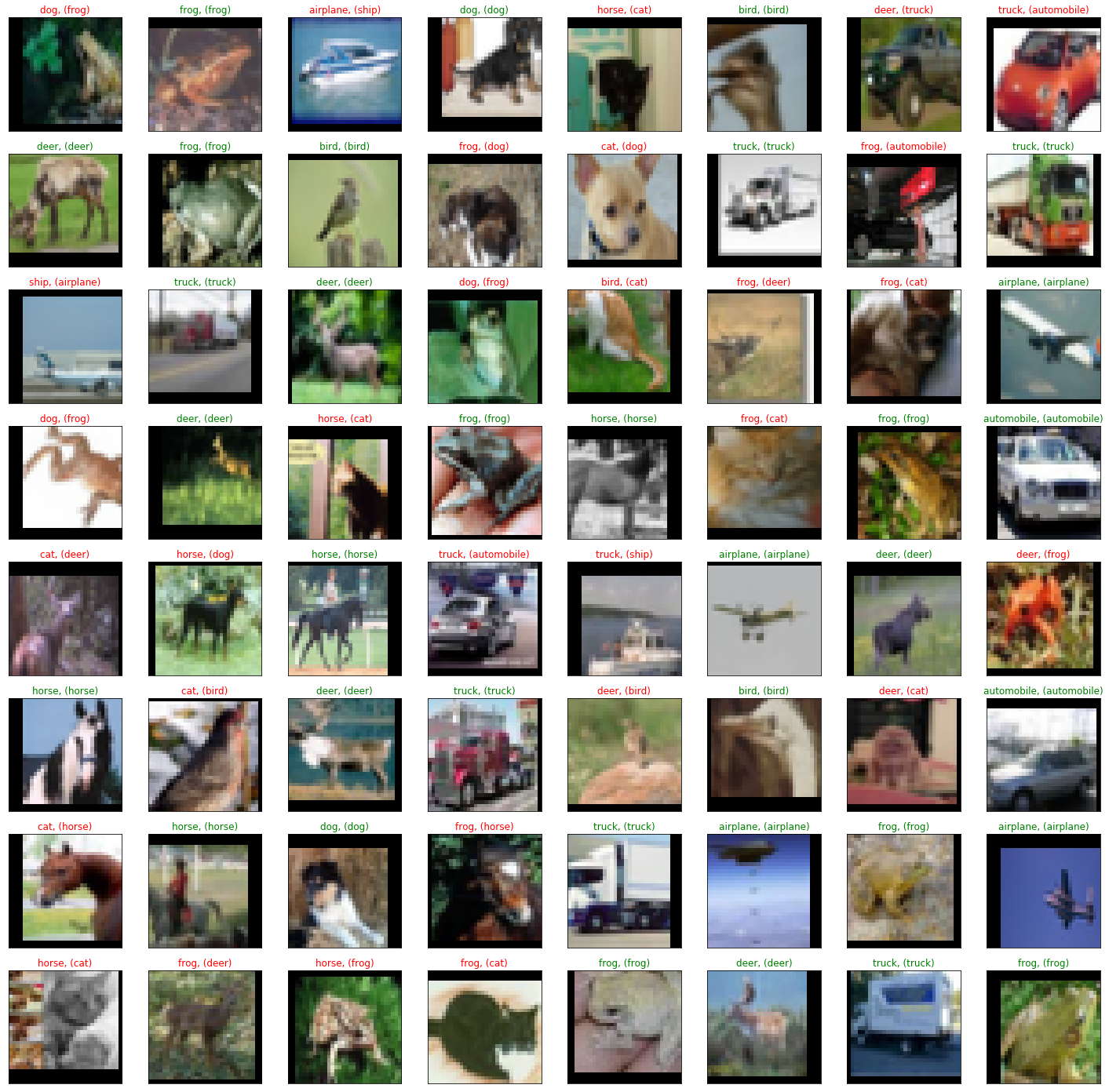
Sample test and visualize some results
dataiter = iter(testloader)
images, labels = dataiter.next()
images_ = images
#images_ = images_.view(images.shape[0], -1)
images_ = images_.to(device)
labels = labels.to(device)
val_output = net(images_)
_, val_preds = torch.max(val_output, 1)

fig = plt.figure(figsize=(25,4))

correct = torch.sum(val_preds == labels.data).item()

val_preds = val_preds.cpu()
labels = labels.cpu()

print("Accuracy Rate = {}%".format(correct/len(images) * 100))

fig = plt.figure(figsize=(25,25))
for idx in np.arange(64):
    ax = fig.add_subplot(8, 8, idx+1, xticks=[], yticks=[])
    #fig.tight_layout()
#     plt.imshow(im_convert(images[idx]))
    imshow(images[idx])
    ax.set_title("{}, ({})".format(classes[val_preds[idx].item()], classes[labels[idx].item()]),
                 color = ("green" if val_preds[idx].item()==labels[idx].item() else "red"))
Accuracy Rate = 58.59375%
<Figure size 1800x288 with 0 Axes>
8. Save model
torch.save(net,save_path[:-4]+'_'+str(epoch)+'.pth')
# torch.save(net, './model/MyNet.pth')
9. Forecast
Read local pictures for prediction
import torch
from PIL import Image
from torch.autograd import Variable
import torch.nn.functional as F
from torchvision import datasets, transforms
import numpy as np

classes = ('plane', 'car', 'bird', 'cat',
           'deer', 'dog', 'frog', 'horse', 'ship', 'truck')

device = torch.device('cuda' if torch.cuda.is_available() else 'cpu')

model = Mynet()

model = torch.load(save_path)  # Loading model
# model = model.to('cuda')
model.eval()  # Change the model to test mode

# Read pictures to predict
img = Image.open("./airplane.jpg").convert('RGB') # Read image
img

Then we will predict the images, but here is a point. We need to transform our images, because we also transform each image during training, so we need to keep consistent
trans = transforms.Compose([transforms.Scale((32,32)),
                            transforms.ToTensor(),
                            transforms.Normalize(mean=(0.5, 0.5, 0.5),
                                                 std=(0.5, 0.5, 0.5)),
                           ])

img = trans(img)
img = img.to(device)
# The picture is expanded to one dimension, because the input into the saved model is 4-dimensional [batch_size, channel, length, width], while the ordinary picture is only three-dimensional, [channel, length, width]
img = img.unsqueeze(0)
    # After expansion, it is [1, 3, 32, 32]
output = model(img)
prob = F.softmax(output,dim=1) #prob is the probability of 10 classifications
print("probability",prob)
value, predicted = torch.max(output.data, 1)
print("category",predicted.item())
print(value)
pred_class = classes[predicted.item()]
print("classification",pred_class)
probability tensor([[8.6320e-01, 1.7801e-04, 3.6034e-03, 3.1733e-04, 2.0015e-03, 6.3802e-05,
      6.5461e-05, 2.0457e-04, 1.2603e-01, 4.3343e-03]], device='cuda:0',
    grad_fn=<SoftmaxBackward>)
Category 0
tensor([6.2719], device='cuda:0')
classification plane
Here we can see that our final result is classified as plane, and our confidence rate is about 86.32%
Read picture address for prediction
We can also predict by reading the url address of the picture. Here I found several different pictures to predict
import requests
from PIL import Image
url = 'https://dss2.bdstatic.com/70cFvnSh_Q1YnxGkpoWK1HF6hhy/it/u=947072664,3925280208&fm=26&gp=0.jpg'
url = 'https://ss0.bdstatic.com/70cFuHSh_Q1YnxGkpoWK1HF6hhy/it/u=2952045457,215279295&fm=26&gp=0.jpg'
url = 'https://ss0.bdstatic.com/70cFvHSh_Q1YnxGkpoWK1HF6hhy/it/u=2838383012,1815030248&fm=26&gp=0.jpg'
url = 'https://gimg2.baidu.com/image_search/src=http%3A%2F%2Fwww.goupuzi.com%2Fnewatt%2FMon_1809%2F1_179223_7463b117c8a2c76.jpg&refer=http%3A%2F%2Fwww.goupuzi.com&app=2002&size=f9999,10000&q=a80&n=0&g=0n&fmt=jpeg?sec=1624346733&t=36ba18326a1e010737f530976201326d'
url = 'https://ss3.bdstatic.com/70cFv8Sh_Q1YnxGkpoWK1HF6hhy/it/u=2799543344,3604342295&fm=224&gp=0.jpg'
# url = 'https://ss1.bdstatic.com/70cFuXSh_Q1YnxGkpoWK1HF6hhy/it/u=2032505694,2851387785&fm=26&gp=0.jpg'
response = requests.get(url, stream=True)
print (response)
img = Image.open(response.raw)
img

It's the same here as before
trans = transforms.Compose([transforms.Scale((32,32)),
                            transforms.ToTensor(),
                            transforms.Normalize(mean=(0.5, 0.5, 0.5),
                                                 std=(0.5, 0.5, 0.5)),
                           ])

img = trans(img)
img = img.to(device)
# The picture is expanded to one dimension, because the input into the saved model is 4-dimensional [batch_size, channel, length, width], while the ordinary picture is only three-dimensional, [channel, length, width]
img = img.unsqueeze(0)
    # After expansion, it is [1, 3, 32, 32]
output = model(img)
prob = F.softmax(output,dim=1) #prob is the probability of 10 classifications
print("probability",prob)
value, predicted = torch.max(output.data, 1)
print("category",predicted.item())
print(value)
pred_class = classes[predicted.item()]
print("classification",pred_class)
probability tensor([[0.7491, 0.0015, 0.0962, 0.0186, 0.0605, 0.0155, 0.0025, 0.0150, 0.0380,
      0.0031]], device='cuda:0', grad_fn=<SoftmaxBackward>)
Category 0
tensor([3.6723], device='cuda:0')
classification plane
It can be seen that the result of our classification is plane, while the real classification is cat, so this model is not particularly perfect and needs to be improved
10. Summary
In fact, for our LeNet5, this model first appeared on the MINST data set, achieved high accuracy, and first used the number recognition on stamps. It can be seen from the experimental results that he does not perform well in the classification of CIFAR10, so if you want to use LeNet5 for image recognition, you should think more about it
Incidentally, our data and codes are described in my summary. If necessary, we can get them ourselves
Here is another summary: Summary