Phase I summary

Tip: it mainly involves combing the ideas of each class and summarizing the usage of python

preface

In the process of learning, I encountered many functions and didn't know how to use them. I checked the data and understood it at that time, but later I forgot it. So I recorded what I learned from scratch for reference.

1, Curriculum development tools

The first phase of the course mainly uses Python, so the Python programming environment needs to be configured

Anaconda and pycham are used for software installation

Tip: Anaconda comes with Jupiter notebooks, so the examples in the course can be opened with Jupiter notebooks
Anaconda is responsible for configuring the python library. Python and Jupiter are visual interfaces for programming
First install Anaconda, Reference tutorial Note that the older Python 3 is used in the course Below 6, tensonflow 1 XX version, so pay attention to the selection of version when configuring. Anaconda has many versions. You need to install the software by yourself. The installation method is to open Anaconda prompt and activate the corresponding configuration. pip install XXX==x.x.x (XXX is the software and x.x.x is the version)
Common versions are attached here
python3.6. Installation of sklearn
numpy-1.16.0
pillow-5.0.0
scipy-1.1.0
scikit_learn-0.19.1
matplotlib-2.2.2
imgaug-0.2.7
tensorflow-1.14
Keras2.2.5
bleach-3.3.0
flask-1.1.2
pandas-1.0.5
moviopy-1.0.0
For convenience, Anaconda's prompt and Jupiter are added to the right-click menu without re typing the command every time. Refer to Add Anaconda Prompt to the right-click menu Finally, you need to change "title Anaconda3" to "title Anaconda3"
When opening the Jupyter switch core, you can refer to Error importing tensorflow in Jupiter Notebook: No module named tensorflow solution So as to switch to its own configured environment; Installation Shapely:OSError: [WinError 126] cannot find the specified module, Reference here In response, the pro test is useful. shapely installed directly by pip lacks a GEOS DLL file, in This website You can find the shapely library corresponding to the python version. There is also a subsequent software installation problem, that is, the autopilot interactive interface cannot autopilot because the socket IO version of communication is inconsistent, Reference here

pip install Flask-SocketIO==4.3.1 
pip install python-engineio==3.13.2 
pip install python-socketio==4.6.0 

2, python function

1.sess.run()

After building the diagram, you need to start the diagram in a session session. The first step is to create a session object.
In order to retrieve the output of the Fetch operation, you can pass in some tensors when using the run() call execution diagram of the Session object. These tensors will help you retrieve the results.
In the python language, the returned tensor is a numpy ndarray object
Use sess There are two situations for run():
(1) When you want to get a variable:
(2) When performing an operation, the operation is not a variable and has no value, as shown in the following figure. n this update operation also includes the optimizer during neural network training:
Function description

2. Distinguish numpy (axis = 0 and axis=1)

In fact, there is a problem understanding axis, DF Mean actually takes the mean value of all columns on each row, rather than retaining the mean value of each column. Perhaps simply remember that axis=0 stands for down, and axis=1 stands for across, as an adverb of method action
let me put it another way:
• use a value of 0 to execute the method down the label \ index value of each column or row
• a value of 1 indicates that the corresponding method is performed along the label direction of each row or column
The following figure represents the meaning when axis is 0 and 1 in DataFrame:
a.sum() is the sum of each element in a
a.sum(axis=0) is to calculate the sum of elements in each column of A. hint: it is to add in the direction of axis=0
a.sum(axis=1) is the sum of elements in each row of A
Function description

3.tf.matmul() and TF Multiply() distinguish

1.tf.multiply() multiplies the corresponding elements of the two matrices
2.tf.matmul() multiplies matrix A by matrix b to generate a * b
Function description

4.tf.truncated_normal()

Interpretation: truncated random number that produces normal distribution, that is, if the difference between the random number and the mean is greater than twice the standard deviation, it will be regenerated.
• shape, which generates the dimension of the tensor
• mean
• stddev, standard deviation
Function description

5.tf.placeholder()

Tensorflow's design concept is called computational flow graph. When writing programs, first build the graph of the whole system, and the code will not take effect directly. This is different from other numerical calculation libraries of python (such as Numpy). Graph is static, similar to the image in docker. Then, in the actual running time, start a session, and the program will really run. The advantage of this is to avoid repeatedly switching the actual running context of the underlying program, and tensorflow helps you optimize the code of the whole system. As we know, the bottom layer of many Python programs is C language or other languages. When executing a line of script, you have to switch once. It is cost-effective. Tensorflow helps you optimize the code to be executed in the whole session by calculating the flow graph.
Therefore, the placeholder() function occupies the position in the model when the neural network constructs the graph. At this time, it does not transfer the data to be input into the model, but only allocates the necessary memory. When the session is established, the feed is used when running the model in the session_ The dict() function feeds data to the placeholder.
Function description

6.np.argmax()

Take out the index corresponding to the maximum value of the element, and return the index corresponding to the maximum value, not the maximum value
Function description

Item 1:

1. Distinguish between blue and white
2. Convert to grayscale image
3. Gaussian filtering: smooth edges to reduce noise
4. Edge detection
5. Regions of interest
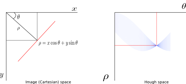
6. Hough transform

Item 2:

It is mainly to set the parameters of each layer of deep neural network

Item 3:

1. Calibrate the camera to obtain the corresponding relationship between the real point and the midpoint of the image RET, corners = CV2 findChessboardCorners()
2. Corrected distortion, RET, MTX, dist, rvecs, tvecs = CV2 Calibratecamera () calibrates the camera matrix and distortion parameters. Rotation and translation vectors, etc., DST = CV2 Undistort (IMG, MTX, dist, none, MTX) corrects distortion
3. Select the features (road lines) in the picture through color, gradient, etc.: color threshold (yellow and white), gradient threshold (X,Y,XY), directional gradient (dir). Use multiple to merge and generate combined
4. Perspective transformation: extract the ladder diagram of the route and transform it into a road diagram with rectangular features
5. Find out the center point of the route by calculating the sum of y direction, and then iterate continuously in the window to find out all the points, second-order fitting NP polyfit(lefty, leftx, 2)
6. Draw the widened road line and green area of the road
7. Combined with video processing

# ffmpeg is responsible for extracting the pictures between 0-4 videos and using a detector for real-time monitoring. The main problem here is how to penetrate the global parameters
# So create the class of AdvancedLaneDetectorWithMemory
from moviepy.video.io.ffmpeg_tools import ffmpeg_extract_subclip
ffmpeg_extract_subclip(challenge_video_path, 0, 4, targetname=challenge_video_path)
detector = AdvancedLaneDetectorWithMemory(opts, ipts, src_pts, dst_pts, 20, 100, 10)
clip1 = VideoFileClip(challenge_video_sample_path)
challenge_video_clip = clip1.fl_image(detector.process_image)  # NOTE: this function expects color images!!
challenge_video_clip.write_videofile(challenge_video_sample_output_path, audio=False)

Item 4:

1. Feature extraction: rsize simplify picture - > (manual) color, direction gradient, extract all features of a picture as a vector, and then arrange all pictures vertically
2. Classifier: a total of three classifiers can be tried: obtain pictures, extract features - > disrupt pictures - > z = (x - U) / s data standardization
X_scaler = StandardScaler().fit(X_train)
Apply the scaler to XX_train = X_scaler.transform(X_train)
Training classifier
3. Sliding window: for each picture, use the sliding window to extract the window features, and then use the trained classifier to predict (identify), and the prediction = 1 will be recorded
4. Finally, the window will be displayed

The following procedures cannot be run directly

Chapter II

This program cannot be run directly
 Read in the picture and choose the color
mpimg.imread('test.jpg')
ysize = image.shape[0]
xsize = image.shape[1]
color_select = np.copy(image)
thresholds = (image[:,:,0] < rgb_threshold[0]) \
            | (image[:,:,1] < rgb_threshold[1]) \ about X[:,:,1]Is to take all the data in the first dimension of the three-dimensional matrix
            | (image[:,:,2] < rgb_threshold[2])
color_select[thresholds] = [0,0,0]
Draw a triangle
fit_left = np.polyfit((left_bottom[0], apex[0]), (left_bottom[1], apex[1]), 1)
fit_right = np.polyfit((right_bottom[0], apex[0]), (right_bottom[1], apex[1]), 1)
fit_bottom = np.polyfit((left_bottom[0], right_bottom[0]), (left_bottom[1], right_bottom[1]), 1)
XX, YY = np.meshgrid(np.arange(0, xsize), np.arange(0, ysize))
region_thresholds = (YY > (XX*fit_left[0] + fit_left[1])) & \
                    (YY > (XX*fit_right[0] + fit_right[1])) & \
                    (YY < (XX*fit_bottom[0] + fit_bottom[1]))
Convert to grayscale image first
gray = cv2.cvtColor(image, cv2.COLOR_RGB2GRAY) #grayscale conversion
 Advanced Gaussian filtering
kernel_size = 3 # Must be an odd number (3, 5, 7...)
blur_gray = cv2.GaussianBlur(gray,(kernel_size, kernel_size),0)
Then edge detection
edges = cv2.Canny(gray, low_threshold, high_threshold) [Reference documents](https://docs.opencv.org/2.4/doc/tutorials/imgproc/imgtrans/canny_detector/canny_detector.html)
Take out the points to fit
cv2.fillPoly(mask, vertices, ignore_mask_color) # vertices are painted on the mask and the color is ignore_mask_color
masked_edges = cv2.bitwise_and(edges, mask)
Finally, Hough transform is used to find the fitting route
lines = cv2.HoughLinesP(masked_edges, rho, theta, threshold, np.array([]),
                            min_line_length, max_line_gap)
cv2.line(line_image,(x1,y1),(x2,y2),(255,0,0),10)
np.dstack((edges, edges, edges))    
# addWeighted is actually an addition, but it is mixed in proportion with different weights, giving people a mixed or transparent feeling     
lines_edges = cv2.addWeighted(color_edges, 0.8, line_image, 1, 0)                                    

Chapter III

# and logic operation
test_inputs = [(0, 0), (0, 1), (1, 0), (1, 1)]
correct_outputs = [False, False, False, True]
outputs = []
for test_input, correct_output in zip(test_inputs, correct_outputs):
    linear_combination = weight1 * test_input[0] + weight2 * test_input[1] + bias
    output = int(linear_combination >= 0)
    is_correct_string = 'Yes' if output == correct_output else 'No'
    outputs.append([test_input[0], test_input[1], linear_combination, output, is_correct_string])

# Print output returns output[4] in the form of a list when output[4] = 'no'
num_wrong = len([output[4] for output in outputs if output[4] == 'No'])
output_frame = pd.DataFrame(outputs, columns=['Input 1', '  Input 2', '  Linear Combination', '  Activation Output', '  Is Correct']) #Use the dataframe of panda to facilitate reading and writing
# OR change to this
test_inputs = [(0, 0), (0, 1), (1, 0), (1, 1)]
correct_outputs = [True, False, True, False]
outputs = []

Chapter IV

# miniflow main parameters
import numpy as np

class Node:
    def __init__(self, inbound_nodes=[]):
        self.inbound_nodes = inbound_nodes
        self.value = None
        self.outbound_nodes = []
        self.gradients = {}
        for node in inbound_nodes:
            node.outbound_nodes.append(self
    def forward(self):
        raise NotImplementedError
    def backward(self):
        raise NotImplementedError

class Input(Node):
    """
    A generic input into the network.
    """
    def __init__(self):
        Node.__init__(self)
    def forward(self):
        pass
    def backward(self):
        self.gradients = {self: 0}
        for n in self.outbound_nodes:
            self.gradients[self] += n.gradients[self]
class Linear(Node):
    """
    Represents a node that performs a linear transform.
    """
    def __init__(self, X, W, b):
        Node.__init__(self, [X, W, b])
    def forward(self):
        X = self.inbound_nodes[0].value
        W = self.inbound_nodes[1].value
        b = self.inbound_nodes[2].value
        self.value = np.dot(X, W) + b
    def backward(self):
        self.gradients = {n: np.zeros_like(n.value) for n in self.inbound_nodes}
        for n in self.outbound_nodes:
            grad_cost = n.gradients[self]
            self.gradients[self.inbound_nodes[0]] += np.dot(grad_cost, self.inbound_nodes[1].value.T)
            self.gradients[self.inbound_nodes[1]] += np.dot(self.inbound_nodes[0].value.T, grad_cost)
            self.gradients[self.inbound_nodes[2]] += np.sum(grad_cost, axis=0, keepdims=False)
class Sigmoid(Node):
    """
    Represents a node that performs the sigmoid activation function.
    """
    def __init__(self, node):
        Node.__init__(self, [node])
    def _sigmoid(self, x):
        return 1. / (1. + np.exp(-x))
    def forward(self):
        input_value = self.inbound_nodes[0].value
        self.value = self._sigmoid(input_value)
    def backward(self):
        self.gradients = {n: np.zeros_like(n.value) for n in self.inbound_nodes}
        for n in self.outbound_nodes:
            grad_cost = n.gradients[self]
            sigmoid = self.value
            self.gradients[self.inbound_nodes[0]] += sigmoid * (1 - sigmoid) * grad_cost
class MSE(Node):
    def __init__(self, y, a):
        """
        The mean squared error cost function.
        Should be used as the last node for a network.
        """
        Node.__init__(self, [y, a])
    def forward(self):
        y = self.inbound_nodes[0].value.reshape(-1, 1)
        a = self.inbound_nodes[1].value.reshape(-1, 1)
        self.m = self.inbound_nodes[0].value.shape[0]
        self.diff = y - a
        self.value = np.mean(self.diff**2)
    def backward(self):      
        self.gradients[self.inbound_nodes[0]] = (2 / self.m) * self.diff
        self.gradients[self.inbound_nodes[1]] = (-2 / self.m) * self.diff
def forward_and_backward(graph):
    """
    Performs a forward pass and a backward pass through a list of sorted Nodes.
    Arguments: `graph`: The result of calling `topological_sort`.
    """
    for n in graph:
        n.forward()
    for n in graph[::-1]:
        n.backward()
def sgd_update(trainables, learning_rate=1e-2):
    """
    Updates the value of each trainable with SGD Arguments:
        `trainables`: A list of `Input` Nodes representing weights/biases.
        `learning_rate`: The learning rate.
    """
    for t in trainables:
        partial = t.gradients[t]
        t.value -= learning_rate * partial

Chapter V

read_data_sets('', one_hot=True)  # Hotkey labels, each with only one 1, and the rest are represented by 0
astype(np.float32) #Conversion type
tf.compat.v1.placeholder() # Predefined parameters
tf.Variable() #TF2.0 assignment method
logits = tf.add(tf.matmul(features, weights), bias) #Matrix multiplication
cost = tf.reduce_mean()  #Mean value of tensor
optimizer = tf.compat.v1.train.GradientDescentOptimizer(learning_rate=learning_rate).minimize(cost) #  The minimize() function handles two operations: gradient calculation and parameter update
tf.equal()
tf.argmax()
init = tf.compat.v1.global_variables_initializer()
with tf.compat.v1.compat.v1.Session() as sess:
    sess.run(init)    
    for batch_features, batch_labels in batches(batch_size, train_features, train_labels):
        sess.run(optimizer, feed_dict={features: batch_features, labels: batch_labels})
    test_accuracy = sess.run( accuracy,feed_dict={features: test_features, labels: test_labels})
print('Test Accuracy: {}'.format(test_accuracy))

Chapter VI

with ZipFile(file) as zipf:  #  There is no need to close the file manually. When the content is executed, the file is automatically closed.
filenames_pbar = tqdm(zipf.namelist(), unit='files')  #  You can use zipfile Namelist () returns the name list of the whole compressed file, and then unzip it one by one to return to the progress bar
if not filename.endswith('/'):  #  Judge whether the file name ends with /. If not, continue
with zipf.open(filename) as image_file:  #  Open a file
image = Image.open(image_file)  #  Picture reading
feature = np.array().flatten()  #  First it becomes a matrix and then it is reduced to a one bit dimension
label = os.path.split(filename)[1][0]  #  Separate file names and paths by path characters
encoder.fit(train_labels) # Binarize the lebals tag
train_labels = encoder.transform(train_labels)  # : on the basis of Fit, carry out standardization, dimension reduction, normalization and other operations
train_test_split(
    train_features,
    train_labels,
    test_size=0.05,  # If it is floating point, it indicates the percentage of the test set in the total sample
    random_state=832289)  # If it is an integer, the data generated each time is the same
assert features._op.name.startswith('Placeholder'), 'features must be a placeholder' # Check whether the feature starts with placeholder
assert labels._op.name.startswith('Placeholder'), 'labels must be a placeholder' # Check whether the feature starts with placeholder
assert isinstance(weights, Variable), 'weights must be a TensorFlow variable'  # isinstance() is used to determine whether an object is of the specified type
cross_entropy = -tf.reduce_sum(labels * tf.math.log(prediction), axis=1)  # Compress the dimension corresponding to axis=1 and reduce the dimension
loss = tf.reduce_mean(cross_entropy) # Average value after dimension reduction
assert not np.count_nonzero(biases_data), 'biases must be zeros'  # Calculate the number of non-zero elements and all non-zero elements
math.ceil(len(train_features) / batch_size))  #  "Round up" math Floor rounded down math Round round
batches[-1] #  Last bit of batches[-1] array
acc_plot.set_ylim([0, 1.0])  #  y-axis range
acc_plot.set_xlim([batches[0], batches[-1]])  #  x-axis range

Chapter VII

np.pad(X_validation, ((0, 0), (2, 2), (2, 2), (0, 0)), 'constant')  # Two rows and two columns of 0 (28 + 2 + 2 = 32) are added at the beginning and end to reach the input of 32 * 32.
index = random.randint(0, len(X_train))  #Returns any integer between parameter 1 and parameter 2
image = X_train[index].squeeze()  #Remove single dimension entries and empty [] shells
X_train, y_train = shuffle(X_train, y_train)  #Disorder order
conv1 = tf.nn.conv2d(x, conv1_W, strides=[1, 1, 1, 1], padding='VALID') + conv1_b
# Convolution matmul is used for gray image and one-dimensional image x: input; conv1_W: filter, convolution kernel, stripes [1, height, weight, 1] padding= valid, do not fill 0
conv1 = tf.nn.relu(conv1) #Activation function
conv1 = tf.nn.max_pool2d(conv1, ksize=[1, 2, 2, 1], strides = [1, 2, 2, 1], padding = 'VALID') #Pooling function, taking the maximum value
fc0 = tf.layers.flatten(conv2) #delayering
one_hot_y = tf.one_hot(y, 10) #Using an eigenvalue 1 to represent different situations, there is only one calorific value
cross_entropy = tf.nn.softmax_cross_entropy_with_logits_v2(labels=one_hot_y, logits=logits) #: 1. Convert logits into probability according to the formula; 2. The calculation result of cross entropy loss is in the form of [0,0,1,0]lebal label
loss_operation = tf.reduce_mean(cross_entropy)  #Calculate average
optimizer = tf.train.AdamOptimizer(learning_rate = rate)  #The name comes from Adaptive Moment Estimation, which is also a deformation of gradient descent algorithm. The advantage is stability
tf.nn.top_k(tf.nn.softmax(self.logits), k=5, sorted=True, name=None)  # In order to find the maximum k values of the last dimension of the input tensor and its subscript!

Chapter IX

from keras.models import Sequential
from keras.layers.core import Dense, Activation, Flatten
from keras.layers.convolutional import Convolution2D

# TODO: Build Convolutional Neural Network in Keras Here
model = Sequential()
model.add(Convolution2D(32, 3, 3, input_shape=(32, 32, 3)))  #
# model.add(Convolution2D(64, 3, 3, border_mode='same', input_shape=(3, 256, 256)))
# The parameter means to take 64 convolution kernels of 3 * 3, retain the convolution result at the boundary (i.e. the output shape is the same as the input shape), and convolute the input data of 3 * 256 * 256.
model.add(MaxPooling2D(pool_size=(2,2),strides=(2,2)))  # Stripe is equal to pool by default_ size
model.add(Dropout(0.5)) # Make some neural network nodes invalid and avoid over fitting
model.add(Activation('relu'))  #  a ReLU activation layer
model.add(Flatten())  
model.add(Dense(128))   # a fully connected layer
model.add(Activation('relu'))  #  a ReLU activation layer
model.add(Dense(5))
model.add(Activation('softmax'))
# Preprocess data
X_normalized = np.array(X_train / 255.0 - 0.5 )
from sklearn.preprocessing import LabelBinarizer
label_binarizer = LabelBinarizer()
y_one_hot = label_binarizer.fit_transform(y_train)
model.compile('adam', 'categorical_crossentropy', ['accuracy'])
history = model.fit(X_normalized, y_one_hot, nb_epoch=3, validation_split=0.2) #The order of segmentation and shuffle is inconsistent, resulting in inconsistent results each time

Chapter 10

# Transfer learning, using AlexNet network
fc7 = AlexNet(resized, feature_extract=True) #The penultimate stop
fc7 = tf.stop_gradient(fc7) #Avoid inverse transfer of gradient function
shape = (fc7.get_shape().as_list()[-1], nb_classes) # The last dimension represents its output [?, 4096]
fc8W = tf.Variable(tf.truncated_normal(shape, stddev=1e-2))
cross_entropy = tf.nn.sparse_softmax_cross_entropy_with_logits(labels=labels, logits=logits)
loss_op = tf.reduce_mean(cross_entropy)
opt = tf.train.AdamOptimizer()
train_op = opt.minimize(loss_op, var_list=[fc8W, fc8b])  
# Gradient update fc8W and fc8b
# 1,Optimizer. In minimize (loss, var_list), the variables involved in calculating loss (assuming var(loss)) are included in var_ List, which is var_ List contains redundant variables, which does not affect the operation of the program, and VaR is not changed in the optimization process_ The value of the variable appears in the list;
# 2. If var_ If the number of variables in the list is less than var(loss), only var will be updated in the optimization process_ The values of those variables in the list and the extra variable values in var(loss) will not change, which is equivalent to fixing the parameter values of a part of the network.
print("%s: %.3f" % (sign_names.loc[inds[-1 - i]][1], output[input_im_ind, inds[-1 - i]]))  #ix is replaced by loc, which means to take out the corresponding index

Chapter XII

images = glob.glob('calibration_wide/GO*.jpg')  # Returns a list of all matching file paths. The path in the directory is the most
for idx, fname in enumerate(images):  # index fname name path
    img = cv2.imread(fname)
    gray = cv2.cvtColor(img, cv2.COLOR_BGR2GRAY) # Change to grayscale
    g = gray.shape[::-1] # Reverse order
    ret, corners = cv2.findChessboardCorners(gray, (8,6), None) # Corners, find the calibrated corner
cv2.drawChessboardCorners(img, (8,6), corners, ret) # Draw corners
ret, mtx, dist, rvecs, tvecs = cv2.calibrateCamera(objpoints, imgpoints, img_size,None,None) # It returns the camera matrix and distortion parameters. Rotation and translation vectors, etc
# mtx: internal parameter matrix
# dist: distortion coefficients=
# rvecs: Rotation vector # External parameters
# tvecs: Translation vector # External parameters
v2.imwrite('calibration_wide/test_undist.jpg',dst) # Save picture
dist_pickle["dist"] = dist
pickle.dump( dist_pickle, open( "calibration_wide/wide_dist_pickle.p", "wb" ) )  # write in. p file
dist_pickle = pickle.load(open( "wide_dist_pickle.p", "rb" )) #Read p file
objpoints = dist_pickle["objpoints"]
M = cv2.getPerspectiveTransform(src, dst) # Obtain transformation parameters
Minv = cv2.getPerspectiveTransform(dst, src)
warped = cv2.warpPerspective(img, M, img_size,flags=cv2.INTER_LINEAR) Change the viewing angle
src = np.float32([corners[0],corners[nx-1],corners[-1],corners[-nx]]).reshape(4,2)  #reshape changes the shape without changing the size. resize changes the number of elements
sobelx = cv2.Sobel(gray, cv2.CV_64F, 1, 0, ksize=sobel_kernel) #It is used to calculate the approximate gradient of image gray. The larger the gradient, the more likely it is to be an edge. The function of Soble operator combines Gaussian smoothing and differential derivation, which is also called first-order differential operator. The derivation operator obtains the gradient image of the image in the X-direction and Y-direction by deriving in the horizontal and vertical directions. Disadvantages: it is sensitive and easy to be affected. Gaussian blur (smoothing) should be used to reduce noise
hls = cv2.cvtColor(image, cv2.COLOR_RGB2HLS) # Convert to HLS space
f, ([ax1, ax2], [ax3, ax4]) = plt.subplots(nrows=2, ncols=2, figsize=(24, 8)) # 2x2 display
f.tight_layout()  #Compact adaptation
ax1.imshow(binary, cmap='gray') #Shaft 1 2 3 4 
ax1.set_title('gray', fontsize=25)
plt.subplots_adjust(left=0., right=1, top=0.9, bottom=0.) # Adjust edge
plt.show() # If it is not written, python will not be displayed
nonzero = binary_warped.nonzero()  # Returns the subscript of a non-zero element, (x,y,z) divided into two matrices
 good_left_inds = ((nonzeroy >= win_y_low) & (nonzeroy < win_y_high) &  (nonzerox >= win_xleft_low) &  (nonzerox < win_xleft_high)).nonzero()[0]  # Take out the tupe element
# Array and element comparison, each element comparison, extract True, and satisfy the x subscript and y subscript in the box
left_fit = np.polyfit(lefty, leftx, 2)  # Second order polynomial fitting
out_img[nonzeroy[left_lane_inds], nonzerox[left_lane_inds]] = [255, 0, 0]  # The corresponding position is attached with color: red
left_line_window1 = np.array([np.transpose(np.vstack([left_fitx - margin, ploty]))])  # Transfer exchange row and column values, similar to transpose
left_line_window2 = np.array([np.flipud(np.transpose(np.vstack([left_fitx + margin, ploty])))])  # Convert to subsequent fill colors, y end to end
left_fit_cr = np.polyfit(ploty*ym_per_pix, leftx*xm_per_pix, 2)
right_fit_cr = np.polyfit(ploty*ym_per_pix, rightx*xm_per_pix, 2)
# Calculate the new radii of curvature
left_curverad = ((1 + (2*left_fit_cr[0]*y_eval*ym_per_pix + left_fit_cr[1])**2)**1.5) / np.absolute(2*left_fit_cr[0])
right_curverad = ((1 + (2*right_fit_cr[0]*y_eval*ym_per_pix + right_fit_cr[1])**2)**1.5) / np.absolute(2*right_fit_cr[0]) #Curvature solution formula

Chapter 13, 14 and 15

xx, yy = np.meshgrid(np.arange(x_min, x_max, h), np.arange(y_min, y_max, h)) # The grid points xx and yy are 100x100 matrix respectively
Z1 = np.c_[xx.ravel(), yy.ravel()]  # Flattening of t ravel array
Z = clf.predict(np.c_[xx.ravel(), yy.ravel()])  # np.c_ Connecting two matrices by row is to add the left and right of the two matrices, and the number of rows is required to be equal
plt.pcolormesh(xx, yy, Z, cmap=pl.cm.seismic)  # The Z range [0,1] corresponds to the color space
output_image("test.png", "png", open("test.png", "rb").read())
def output_image(name, format, bytes):
    image_start = "BEGIN_IMAGE_f9825uweof8jw9fj4r8"
    image_end = "END_IMAGE_0238jfw08fjsiufhw8frs"
    data = {}
    data['name'] = name
    data['format'] = format
    data['bytes'] = base64.encodebytes(bytes).decode('utf-8') # Binary files must be processed in this way to use json
    print(image_start+json.dumps(data)+image_end)
grade_sig = [X_train[ii][0] for ii in range(0, len(X_train)) if y_train[ii]==0]  # There are two lists for each cell. Separate data of grade and bunpy are listed respectively. At this time, y=0
random.seed(42)  #Generate random number seed
grade = [random.random() for ii in range(0,n_points)] # Generate random number seeds in grade bump and error, and each generates 1000 random numbers
# Naive Bayes
from sklearn.naive_bayes import GaussianNB
from sklearn.metrics import accuracy_score
clf = GaussianNB()
clf.fit(features_train,labels_train)
pred = clf.predict(features_test)
accuracy = accuracy_score(labels_test, pred)
# Support vector machine
from sklearn.svm import SVC
clf = SVC(C=10,kernel='linear')
clf.fit(features_train, labels_train)
pred = clf.predict(features_test)
acc = accuracy_score(pred, labels_test)
# Search best
from sklearn import svm 
from sklearn.model_selection import GridSearchCV
parameters = {'kernel':('linear', 'rbf'), 'C':[1, 10]}
svr = svm.SVC()
clf1 = GridSearchCV(svr, parameters)
clf1.fit(features_train, labels_train)
print(clf1.best_params_, clf1.best_score_)
#Decision tree
from sklearn.tree import DecisionTreeClassifier
clf = DecisionTreeClassifier()
clf.fit(features_train, labels_train)
pred = clf.predict(features_test)

Chapter 16

result = cv2.matchTemplate(imcopy, temp, method=cv2.TM_CCOEFF_NORMED)
(minVal, maxVal, minLoc, maxLoc) = cv2.minMaxLoc(result)  # Search for matching pictures and apply TM_CCOEFF returns the maximum corner
# Calculate the histogram of RGB channel respectively
rhist = np.histogram(img[:,:,0], bins=nbins, range=bins_range)  # Then return a tuple (frequency, boundary of sub box), as shown above. It should be noted that the number of this boundary is one more than the number of score boxes, which can be simply confirmed by the following code.
# Generate bin Center
bin_edges = rhist[1]
bin_centers = (bin_edges[1:] + bin_edges[0:len(bin_edges) - 1]) / 2
# The histogram is connected into a single feature vector
hist_features = np.concatenate((rhist[0], ghist[0], bhist[0]))
#Draw histogram
    fig = plt.figure(figsize=(12,3))
    plt.subplot(131)
    plt.bar(bincen, rh[0]) # In bin_center displays the histogram as the center
    plt.xlim(0, 256)
    plt.title('R Histogram')
features = cv2.resize(feature_image, size).ravel() # Simplify the size and transform it into a feature vector
features, hog_image=hog(img, orient, (pix_per_cell,pix_per_cell), (cell_per_block,cell_per_block),block_norm='L1', visualize=vis, feature_vector=feature_vec) # Obtain gradient
X = np.vstack((car_features, notcar_features)).astype(np.float64)    # Stack each list vertically to get the matrix
np.concatenate(img_features)  # Become a line
cv2.rectangle(draw_img,(xbox_left, ytop_draw+ystart),(xbox_left+win_draw,ytop_draw+win_draw+ystart),(0,0,255),6) # Draw rectangle
X_train = X_scaler.transform(X_train)  # Find X_ The mean and standard deviation of train are used in X_ z = (x - u) / s on the train. For each attribute / column, all data are clustered near 0, and the standard deviation is 1, so that the variance of the new x data set is 1 and the mean value is 0
heatmap = np.clip(heat, 0, 255) #It means that all the numbers less than min are replaced with min, all the numbers greater than max are replaced with Max, and the numbers between [min,max] remain unchanged
**be careful**
matplotlib image will read these in on a scale of 0 to 1, but cv2.imread() will scale them from 0 to 255，if you take an image that is scaled from 0 to 1 and change color spaces using cv2.cvtColor() you'll get back an image scaled from 0 to 255
# Generators are a good way to handle large amounts of data. Using the generator, you can extract data fragments and process them dynamically only when needed, rather than storing all the preprocessed data in memory at one time, so that the memory efficiency is higher. The generator is like a coroutine, a process that can run separately from another main program, which makes it a useful Python function. return generator does not use yield
def fibonacci():
    numbers_list = []
    while 1:
        if(len(numbers_list) < 2):
            numbers_list.append(1)
        else:
            numbers_list.append(numbers_list[-1] + numbers_list[-2])
        yield 1 # change this line so it yields its list instead of 1
our_generator = fibonacci()
my_output = []
for i in range(10):
    my_output = (next(our_generator))
# usage method
def generator(samples, batch_size=32)
train_generator = generator(train_samples, batch_size=32)
model.fit_generator(train_generator, samples_per_epoch= len(train_samples),
validation_data=validation_generator,nb_val_samples=len(validation_samples), nb_epoch=3)
np.asarray(list(map(lambda path: load_image(path),  np.asarray(project_vehicle_img_paths)[np.random.randint(0, high=len(project_vehicle_img_paths), size=5)]) # lambda, which simplifies the execution of functions on each element

Imported Library

import matplotlib. Pyplot as plot # import drawing library
import matplotlib.image as mpimg # image processing
import hashlib # hash algorithm
import os # import standard library
import pickle # data persistence
from urllib.request import urlretrieve # remote data download to local
import numpy as np # array processing library
from PIL import Image # image processing library
from sklearn.model_selection import train_test_split # randomly divides the sample data into training set and test set
from sklearn.preprocessing import LabelBinarizer # label binarization
from sklearn.utils import resample # resample
from tqdm import tqdm # progress bar
from zipfile import ZipFile # zip format encoding compression and decompression