Pytoch: fast migration of image style - residual network, fixed style and arbitrary content
Copyright: Jingmin Wei, Pattern Recognition and Intelligent System, School of Artificial and Intelligence, Huazhong University of Science and Technology
This tutorial is not for commercial use. It is only for learning and reference. If you need to reprint it, please contact me.
Reference
Perceptual Losses for Real-Time Style Transfer and Super-Resolution
Unlike ordinary style migration, the input image of ordinary image style migration is random noise, while the input of fast style migration is an image conversion network f w fw fw output.
Fast style migration is through the input image x x x through image conversion network f w fw fw, get the output of the network y ^ \hat{y} y^ . Therefore, it can realize fast image migration of arbitrary content.
Refer to the article perceptual losses for real time style transfer and super resolution to adjust the up sampling operation of the image conversion network accordingly. In the established network, the transpose convolution operation will be used for up sampling of feature mapping.
import numpy as np
import pandas as pd
import matplotlib.pyplot as plt
from PIL import Image
import time

import torch
import torch.nn as nn
import torch.utils.data as Data
import torch.nn.functional as F
import torch.optim as optim
from torchvision import transforms
from torchvision.datasets import ImageFolder
from torchvision import models
import os
os.environ["KMP_DUPLICATE_LIB_OK"]="TRUE"

# Select GPU for model loading
device = torch.device("cuda" if torch.cuda.is_available() else "cpu")
# device = torch.device('cpu')
print(device)
print(torch.cuda.device_count())
print(torch.cuda.get_device_name(0))
cuda
1
GeForce MX250
Fast style migration network preparation
adopt 3 3 Three convolution layers reduce the dimension of the image feature mapping, and then 5 5 Five residual connection layers, learn the image style and add it to the content image. Finally, through 3 3 Three transpose convolution operations are used to upgrade the dimension of the feature map (analogous to the semantic segmentation network) to reconstruct the image after style migration.
In the dimension upgrading operation of the conversion network, transpose convolution is used to replace the combination of up sampling and convolution layer in the article, because the input is the standardized image, and the pixel value range is − 2.1 − 2.7 -2.1-2.7 − 2.1 − 2.7, so in the last output layer of the network, the activation function is not used, and most of the output values of the network will be in − 2.1 − 2.7 -2.1-2.7 Between − 2.1 − 2.7, only a small part is not in this interval, so when actually training the network, the output will be cut to − 2.1 − 2.7 -2.1-2.7 Between − 2.1 − 2.7, that is, the last layer does not need to use the activation function, and other layers use the ReLU function. In the network, the number of feature maps gradually changes from 3 3 3 added to 128 128 128, and each residual connection layer has 128 128 128 feature maps, and the number of feature maps in the transposed convolution layer will increase from 128 128 128 down to 3 3 3. Three channels corresponding to the image.
Structural block definition residuals
Focus on the local of neural network. Set the input to X. Suppose that the ideal mapping we want to learn is f(x), which is used as the input of the activation function. The part needs to fit the residual mapping f(x) − X of identity mapping. Residual mapping is often easier to optimize in practice. Take identity mapping as the ideal mapping f(x) we want to learn. We only need to learn the weight and deviation parameters of weighting operations (such as affine) 0 0 0, then f(x) is an identity map. In practice, when the ideal mapping f(x) is very close to the identity mapping, the residual mapping is also easy to capture the subtle fluctuations of the identity mapping. In the residual block, the input can propagate forward faster through cross layer data lines.
Define residual connection network, 128 128 128 feature maps, active size 128 × 64 × 64 128\times64\times64 128×64×64
# ResidualBlock residual block
class ResidualBlock(nn.Module):
    def __init__(self, channels):
        super(ResidualBlock, self).__init__()
        self.conv = nn.Sequential(
            nn.Conv2d(channels, channels, kernel_size = 3, stride = 1, padding = 1),
            nn.ReLU(),
            nn.Conv2d(channels, channels, kernel_size = 3, stride = 1, padding = 1)
        )
    def forward(self, x):
        return F.relu(self.conv(x) + x)
Define image conversion network
The lower sampling module, 5 5 Five residual connection modules and up sampling module
# Define image conversion network
class ImfwNet(nn.Module):
    def __init__(self):
        super(ImfwNet, self).__init__()
        # Down sampling
        self.downsample = nn.Sequential(
            nn.ReflectionPad2d(padding = 4), # Use boundary reflection fill
            nn.Conv2d(3, 32, kernel_size = 9, stride = 1),
            nn.InstanceNorm2d(32, affine = True), # Normalize pixel values
            nn.ReLU(),
            nn.Conv2d(32, 64, kernel_size = 3, stride = 2),
            nn.InstanceNorm2d(64, affine = True),
            nn.ReLU(),
            nn.ReflectionPad2d(padding = 1),
            nn.Conv2d(64, 128, kernel_size = 3, stride = 2),
            nn.InstanceNorm2d(128, affine = True),
            nn.ReLU()
        )
        # 5 residual connections
        self.res_blocks = nn.Sequential(
            ResidualBlock(128),
            ResidualBlock(128),
            ResidualBlock(128),
            ResidualBlock(128),
            ResidualBlock(128),
        )
        # Up sampling
        self.unsample = nn.Sequential(
            nn.ConvTranspose2d(128, 64, kernel_size = 3, stride = 2, padding = 1, output_padding = 1),
            nn.InstanceNorm2d(64, affine = True),
            nn.ReLU(),
            nn.ConvTranspose2d(64, 32, kernel_size = 3, stride = 2, padding = 1, output_padding = 1),
            nn.InstanceNorm2d(32, affine = True),
            nn.ReLU(),
            nn.ConvTranspose2d(32, 3, kernel_size = 9, stride = 1, padding = 4)
        )
    def forward(self, x):
        x = self.downsample(x) # The input pixel value is between - 2.1-2.7
        x = self.res_blocks(x)
        x = self.unsample(x) # The output pixel value is between - 2.1-2.7
        return x
myfwnet = ImfwNet().to(device)
from torchsummary import summary
summary(myfwnet, input_size=(3, 256, 256))
----------------------------------------------------------------
        Layer (type)               Output Shape         Param #
================================================================
   ReflectionPad2d-1          [-1, 3, 264, 264]               0
            Conv2d-2         [-1, 32, 256, 256]           7,808
    InstanceNorm2d-3         [-1, 32, 256, 256]              64
              ReLU-4         [-1, 32, 256, 256]               0
            Conv2d-5         [-1, 64, 127, 127]          18,496
    InstanceNorm2d-6         [-1, 64, 127, 127]             128
              ReLU-7         [-1, 64, 127, 127]               0
   ReflectionPad2d-8         [-1, 64, 129, 129]               0
            Conv2d-9          [-1, 128, 64, 64]          73,856
   InstanceNorm2d-10          [-1, 128, 64, 64]             256
             ReLU-11          [-1, 128, 64, 64]               0
           Conv2d-12          [-1, 128, 64, 64]         147,584
             ReLU-13          [-1, 128, 64, 64]               0
           Conv2d-14          [-1, 128, 64, 64]         147,584
    ResidualBlock-15          [-1, 128, 64, 64]               0
           Conv2d-16          [-1, 128, 64, 64]         147,584
             ReLU-17          [-1, 128, 64, 64]               0
           Conv2d-18          [-1, 128, 64, 64]         147,584
    ResidualBlock-19          [-1, 128, 64, 64]               0
           Conv2d-20          [-1, 128, 64, 64]         147,584
             ReLU-21          [-1, 128, 64, 64]               0
           Conv2d-22          [-1, 128, 64, 64]         147,584
    ResidualBlock-23          [-1, 128, 64, 64]               0
           Conv2d-24          [-1, 128, 64, 64]         147,584
             ReLU-25          [-1, 128, 64, 64]               0
           Conv2d-26          [-1, 128, 64, 64]         147,584
    ResidualBlock-27          [-1, 128, 64, 64]               0
           Conv2d-28          [-1, 128, 64, 64]         147,584
             ReLU-29          [-1, 128, 64, 64]               0
           Conv2d-30          [-1, 128, 64, 64]         147,584
    ResidualBlock-31          [-1, 128, 64, 64]               0
  ConvTranspose2d-32         [-1, 64, 128, 128]          73,792
   InstanceNorm2d-33         [-1, 64, 128, 128]             128
             ReLU-34         [-1, 64, 128, 128]               0
  ConvTranspose2d-35         [-1, 32, 256, 256]          18,464
   InstanceNorm2d-36         [-1, 32, 256, 256]              64
             ReLU-37         [-1, 32, 256, 256]               0
  ConvTranspose2d-38          [-1, 3, 256, 256]           7,779
================================================================
Total params: 1,676,675
Trainable params: 1,676,675
Non-trainable params: 0
----------------------------------------------------------------
Input size (MB): 0.75
Forward/backward pass size (MB): 246.85
Params size (MB): 6.40
Estimated Total Size (MB): 253.99
----------------------------------------------------------------
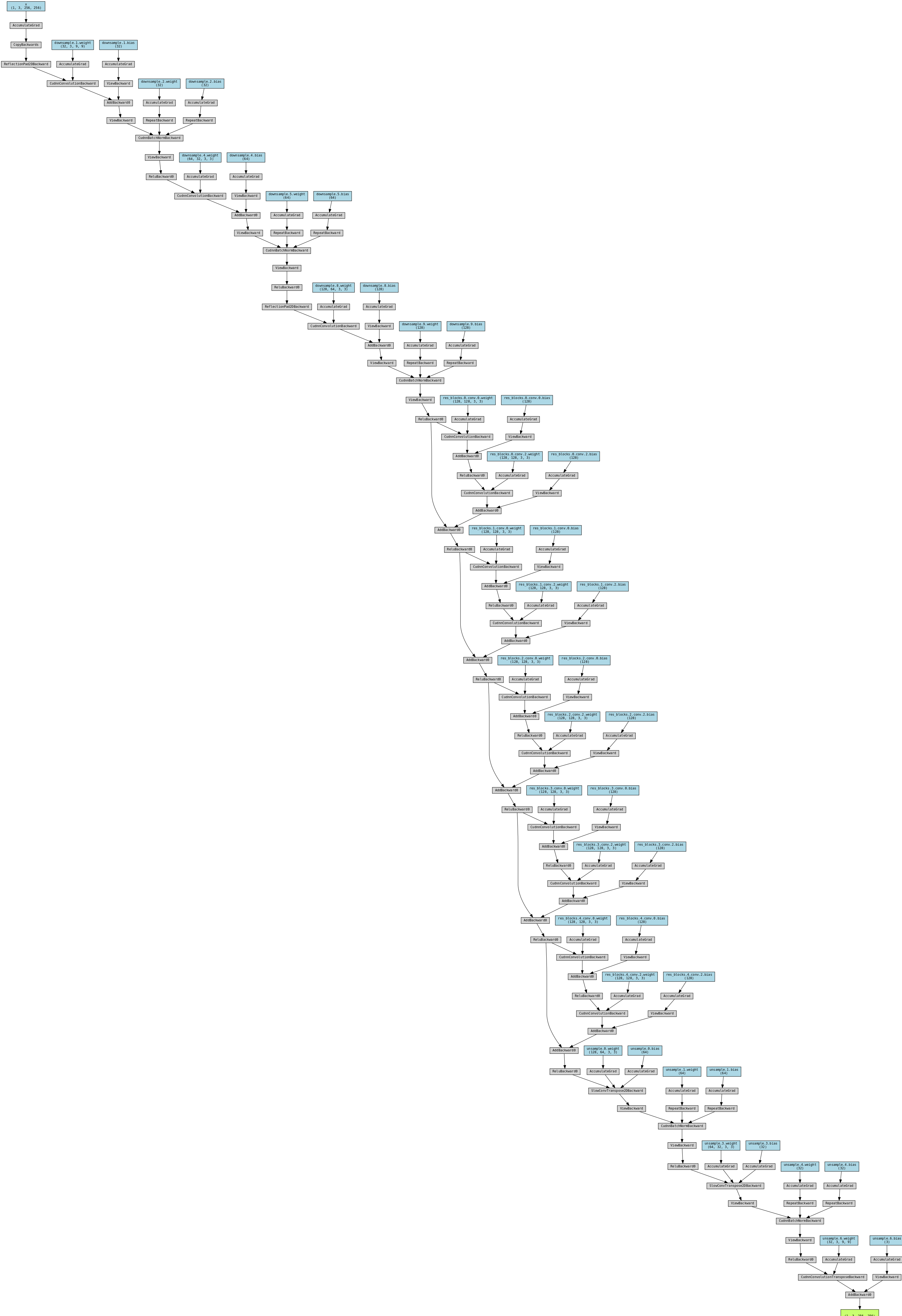
# Output network structure
from torchviz import make_dot

x = torch.randn(1, 3, 256, 256).requires_grad_(True)
y = myfwnet(x.to(device))
myResNet_vis = make_dot(y, params=dict(list(myfwnet.named_parameters()) + [('x', x)]))
myResNet_vis
Fast style migration data preparation
Download address: https://cocodataset.org/#home
The validation set of COCO2014 is used as model input.
# Define image preprocessing
data_transform = transforms.Compose([
    transforms.Resize(256),
    transforms.CenterCrop(256), # The image size is 256 * 256
    transforms.ToTensor(), # Tensor converted to 0-1
    transforms.Normalize(mean = [0.485, 0.456, 0.406],
                         std = [0.229, 0.224, 0.225])
                         # The pixel value is changed to -2.1-2.7
])
# Read data from folder
dataset = ImageFolder('./data/COCO', transform = data_transform)
# Each batch uses 4 images
data_loader = Data.DataLoader(dataset, batch_size = 4, shuffle = True,
                              num_workers = 8, pin_memory = True)
dataset
Dataset ImageFolder
    Number of datapoints: 40504
    Root location: ./data/COCO
    StandardTransform
Transform: Compose(
               Resize(size=256, interpolation=bilinear)
               CenterCrop(size=(256, 256))
               ToTensor()
               Normalize(mean=[0.485, 0.456, 0.406], std=[0.229, 0.224, 0.225])
           )
Description: parameter pin_memory means that when creating a DataLoader, the Tensor data generated first belongs to the lock page memory in memory (all the video memory in the graphics card is lock page memory), so it will be faster to transfer the Tensor of memory to the video memory of GPU, and the operation speed for high-performance GPU will be faster.
Next, read the pre trained VGG16 network, only need the layer contained in the features, and set it to the GPU device. In the calculation, we only need to use VGG network to extract the feature map of a specific layer, without training the parameters, and set it to eval
# Read pre trained VGG16 network
vgg16 = models.vgg16(pretrained = True)
# No classifier is needed, only convolution layer and pooling layer are needed
vgg = vgg16.features.to(device).eval()
Define a method that can read style images and convert them to a four-dimensional tensor format that can be used by VGG networks.
# Define a reading style image function and convert the image as necessary
def load_image(img_path, shape = None):
    image = Image.open(img_path)
    size = image.size
    if shape is not None:
        size = shape # If the image size is specified, it is converted to the specified size
    # Use transforms to convert the image into tensor and standardize it
    in_transform = transforms.Compose([
        transforms.Resize(size),
        transforms.ToTensor(), # Tensor converted to 0-1
        transforms.Normalize(mean = [0.485, 0.456, 0.406],
                            std = [0.229, 0.224, 0.225])
    ])
    # Use the RGB channel of the image and add the batch dimension
    image = in_transform(image)[:3, :, :].unsqueeze(dim = 0)
    return image
# Define a function to convert the standardized image into a visual function using matplotlib
def im_convert(tensor):
    '''
    take[1, c, h, w]The tensor of dimension is transformed into[h, w, c]Array of
    Because the tensor is transformed into a table, it is necessary to carry out standardized inverse transformation
    '''
    tensor = tensor.cpu()
    image = tensor.data.numpy().squeeze() # Remove data from batch dimension
    image = image.transpose(1, 2, 0) # Permutation dimension [C, W, H -] [C, H]
    # Conduct standardized reverse operation
    image = image * np.array((0.229, 0.224, 0.225)) + np.array((0.485, 0.456, 0.406))
    image = image.clip(0, 1) # Cut the value of the image to 0-1
    return image
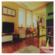
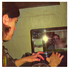
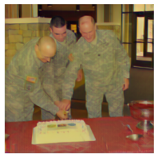
Read style image and visualize
# Read style image
style = load_image('./data/COCO/COCO/COCO_val2014_000000000139.jpg', shape = (256, 256)).to(device)
# Visual image
plt.figure()
plt.imshow(im_convert(style))
plt.axis('off')
plt.show()
Fast style migration network training and data visualization display
As with ordinary style migration, first calculate the Gram matrix of the input tensor:
# Define and calculate Gram matrix
def gram_matrix(tensor):
    '''
    Calculate the image style features Gram Matrix, which can ultimately ensure the content,
    Carry out style transmission. tensor: It is a layer of feature mapping after forward calculation of an image
    '''
    # Obtain the batch of tensor_ size, channel, height, width
    b, c, h, w = tensor.size()
    # Change the dimension of the matrix to (depth, height * width)
    tensor = tensor.view(b, c, h * w)
    tensor_t = tensor.transpose(1, 2)
    # Calculate gram matrix for multiple images
    gram = tensor.bmm(tensor_t) / (c * h * w)
    return gram
Note that since the input data uses a batch feature mapping, when the tensor is multiplied by its transpose, it is necessary to calculate the Gram matrix of each image, so tensor is used BMM method completes the related matrix multiplication calculation
Define get features to obtain the feature mapping of image data on the specified layer of the specified network:
# Defines a method for obtaining the output of an image at a specified layer on the network
def get_features(image, model, layers = None):
    '''
    Put an image image In a network model Forward propagation calculation in,
    And get the specified layer layers Feature output in
    '''
    # Match the name of the mapping layer with the name in the paper
    if layers is None:
        layers = {'3': 'relu1_2',
                  '8': 'relu2_2',
                  '15': 'relu3_3', # Content layer representation
                  '22': 'relu4_3'} # Output after ReLU activation
    features = {} # The obtained features of each layer are saved in the dictionary
    x = image # The image of the feature needs to be acquired
    # model._modules is a dictionary that holds the information of each layer of the network model
    for name, layer in model._modules.items():
        # The features of the image are obtained from the first layer
        x = layer(x)
        # If it is the feature specified by the layers parameter, it is saved to features
        if name in layers:
            features[layers[name]] = x
    return features
Thereinto, relu3_ The feature mapping output from layer 3 is used to measure the similarity of image content.
Next, calculate the style of the image 4 4 4 Gram matrices on the specified multiple layers and save them in a dictionary
# Style representation of computational style image
style_layer = {'3': 'relu1_2',
               '8': 'relu2_2',
               '15': 'relu3_3',
               '22': 'relu4_3'}
content_layer = {'15': 'relu3_3'}
# The layers represented by content use the output after relu activation
style_features = get_features(style, vgg, layers = style_layer)
# Calculate the Gram matrix of each layer for our style representation and save it in a dictionary
style_grams = {layer: gram_matrix(style_features[layer]) for layer in style_features}
Next, start training the network. In the training process, three kinds of losses are defined: style loss, content loss and total variation loss. Their weight is 1 0 5 , 1 , 1 0 − 5 10^5,1,10^{-5} 105,1,10 − 5, the optimizer is Adam, and the learning rate is 0.0003 0.0003 0.0003 . in the light of 4 4 More than 40000 image data, each 4 4 Four images are a batch for training 4 4 4 epoch s, i.e. about 40000 40000 40000 iterations.
# Network training, define the weight of three kinds of losses
style_weight = 1e5
content_weight = 1
tv_weight = 1e-5
# Define optimizer
optimizer = optim.Adam(myfwnet.parameters(), lr = 1e-3)
myfwnet.train()
since = time.time()
for epoch in range(4):
print('Epoch: {}'.format(epoch + 1))
content_loss_all = []
style_loss_all = []
tv_loss_all = []
all_loss = []
for step, batch in enumerate(data_loader):
optimizer.zero_grad()
# Calculate the output of the content image after using the image conversion network
content_images = batch[0].to(device)
transformed_images = myfwnet(content_images)
transformed_images = transformed_images.clamp(-2.1, 2.7)
# Use VGG16 to calculate the content corresponding to the original image_ Layer features
content_features = get_features(content_images, vgg, layers = content_layer)
# Use VGG16 to calculate all features corresponding to the \ hat{y} image
transformed_features = get_features(transformed_images, vgg)
# Content loss
# Use f.mse_ The loss function calculates the loss between transformed_images and content_images
content_loss = F.mse_loss(transformed_features['relu3_3'], content_features['relu3_3'])
content_loss = content_weight * content_loss
# Total variation loss
# The image is horizontally and vertically shifted by one pixel and subtracted from the original image
# Then calculate the sum of the absolute values, which is tv_loss
y = transformed_images # \hat{y}
tv_loss = torch.sum(torch.abs(y[:, :, :, :-1] - y[:, :, :, 1:])) + torch.sum(torch.abs(y[:, :, :-1, :] - y[:, :, 1:, :]))
tv_loss = tv_weight * tv_loss
# Style loss
style_loss = 0
transformed_grams = {layer: gram_matrix(transformed_features[layer]) for layer in transformed_features}
for layer in style_grams:
transformed_gram = transformed_grams[layer]
# Is a Gram for a batch image
style_gram = style_grams[layer]
# It is for an image, so we need to expand the style_gram
# And calculate the loss between transformed_gram and style_gram
style_loss += F.mse_loss(transformed_gram,
style_gram.expand_as(transformed_gram))
style_loss = style_weight * style_loss
# The three losses add up and the gradient decreases
loss = style_loss + content_loss + tv_loss
loss.backward(retain_graph = True)
optimizer.step()
# Count the changes of each loss
content_loss_all.append(content_loss.item())
style_loss_all.append(style_loss.item())
tv_loss_all.append(tv_loss.item())
all_loss.append(loss.item())
if step % 5000 == 0:
print('step: {}; content loss: {:.3f}; style loss: {:.3f}; tv loss: {:.3f}, loss: {:.3f}'.format(step, content_loss.item(), style_loss.item(), tv_loss.item(), loss.item()))
time_use = time.time() - since
print('Train complete in {:.0f}m {:.0f}s'.format(time_use // 60, time_use % 60))
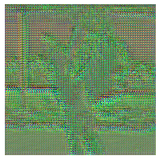
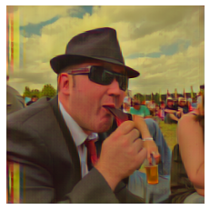
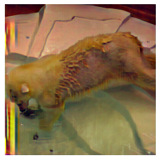
# Visualize an image
plt.figure()
im = transformed_images[1, ...] # The ellipsis indicates that the following contents are not written
plt.axis('off')
plt.imshow(im_convert(im))
plt.show()
Epoch: 1
step: 0; content loss: 21.736; style loss: 679.825; tv loss: 17.357, loss: 718.918
Train complete in 0m 10s
step: 5000; content loss: 11.223; style loss: 4.921; tv loss: 1.068, loss: 17.212
Train complete in 32m 21s
step: 10000; content loss: 10.715; style loss: 3.768; tv loss: 1.101, loss: 15.584
Train complete in 64m 34s
Epoch: 2
step: 0; content loss: 12.664; style loss: 3.324; tv loss: 1.182, loss: 17.170
Train complete in 65m 40s
step: 5000; content loss: 5.582; style loss: 3.621; tv loss: 1.234, loss: 10.438
Train complete in 97m 55s
step: 10000; content loss: 5.797; style loss: 3.302; tv loss: 1.209, loss: 10.308
Train complete in 130m 11s
Epoch: 3
step: 0; content loss: 4.639; style loss: 3.312; tv loss: 1.250, loss: 9.201
Train complete in 131m 16s
step: 5000; content loss: 4.507; style loss: 3.565; tv loss: 1.291, loss: 9.364
Train complete in 163m 32s
step: 10000; content loss: 4.570; style loss: 3.609; tv loss: 1.098, loss: 9.276
Train complete in 195m 48s
Epoch: 4
step: 0; content loss: 4.425; style loss: 2.844; tv loss: 1.239, loss: 8.509
Train complete in 196m 46s
step: 5000; content loss: 6.227; style loss: 4.176; tv loss: 1.231, loss: 11.633
Train complete in 229m 2s
step: 10000; content loss: 4.537; style loss: 3.191; tv loss: 1.178, loss: 8.906
Train complete in 261m 19s
# Save the trained network myfwnet
torch.save(myfwnet.state_dict(), './model/imfwnet_dict.pkl')
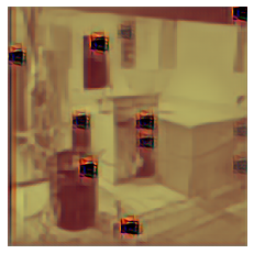
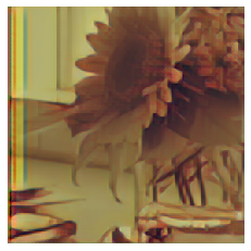
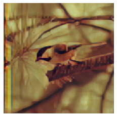
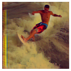
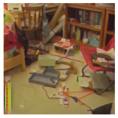
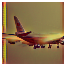
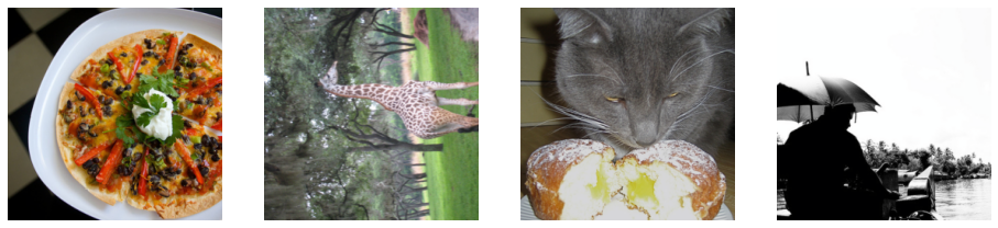
In order to test the style migration network fwnet obtained from training, the following randomly obtains the image of a batch in the data set for image style migration:
myfwnet.eval()
for step, batch in enumerate(data_loader):
content_images = batch[0].to(device)
if step > 0:
break
plt.figure(figsize = (16, 4))
for ii in range(4):
im = content_images[ii, ...]
plt.subplot(1, 4, ii + 1)
plt.axis('off')
plt.imshow(im_convert(im))
plt.show()
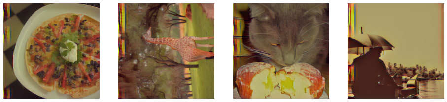
transformed_images = myfwnet(content_images)
transformed_images = transformed_images.clamp(-2.1, 2.7)
plt.figure(figsize = (16, 4))
for ii in range(4):
im = im_convert(transformed_images[ii, ...])
plt.subplot(1, 4, ii + 1)
plt.axis('off')
plt.imshow(im)
plt.show()
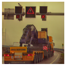
Use the GPU pre training model
# Read content image
content = load_image('./data/COCO/COCO/COCO_val2014_000000000192.jpg', shape = (256, 256))
# Import the trained GPU network
device = torch.device('cpu')
newfwnet = ImfwNet()
newfwnet.load_state_dict(torch.load('./model/imfwnet_dict.pkl', map_location = device)) # The GPU model is mapped to a network based on CPU computing
transform_content = newfwnet(content)
# Visual image
plt.figure()
plt.subplot(1, 2, 1)
plt.imshow(im_convert(content))
plt.axis('off')
plt.subplot(1, 2, 2)
plt.imshow(im_convert(transform_content))
plt.axis('off')
plt.show()
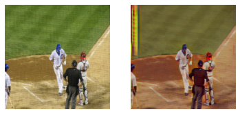
Generally speaking, common style migration takes a long time (it will take several hours), but the effect of style migration is good.
Fast style migration is very fast (the network has been trained, which is an offline process), but the effect is not so ideal.