Pytorch:Hollow Convolution Neural Network
Copyright: Jingmin Wei, Pattern Recognition and Intelligent System, School of Artificial and Intelligence, Huazhong University of Science and Technology
This tutorial is not commercial and is only for learning and reference exchange. If you need to reproduce it, please contact me.
Void convolution adds voids to the convolution core as opposed to ordinary convolution. 0 0 0 element), thereby increasing the field of feeling and getting more information. Reception fields are the area sizes of the input layer corresponding to an element in the output of a layer in a convolution neural network. A common explanation is that a point on the feature map corresponds to the area size on the input graph.
For a 3 × 3 3\times3 3 × 3 2 2 2-Void convolution, the actual convolution kernel size or 3 × 3 3\times3 3 × 3. But the void is 1 1 1, so the convolution kernel expands one 7 × 7 7\times7 7 × 7 image blocks, but only 9 9 Nine red points will have weights to convolute. It can also be understood that the size of the convolution kernel is 7 × 7 7\times7 7 × 7, but only in the diagram 9 9 9 points do not have a weight of 0 0 0, all others are 0 0 0. The actual convolution weight is only 3 × 3 3\times3 3 × 3, but the receptive field is actually 7 × 7 7\times7 7 × 7. about 15 × 15 15\times15 15 × 15, the actual convolution is only 9 × 9 9\times9 9×9 .
At nn. In the Conv2d() function, by adjusting the value of dilation, the void convolution of convolution kernels of different sizes can be performed.
The void convolution network we built has two void convolution layers, two pooling layers and two fully connected layers, and the classifier still contains 10 10 Ten neurons, with the exception of differences in convolution modes, share the same network structure as the one used to identify FashionMNIST.
Construction of Hole Convolution Neural Network
import numpy as np
import pandas as pd
from sklearn.metrics import accuracy_score, confusion_matrix
import matplotlib.pyplot as plt
import seaborn as sns
import copy
import time
import torch
import torch.nn as nn
from torch.optim import Adam
import torch.utils.data as Data
from torchvision import transforms
from torchvision.datasets import FashionMNIST
class MyConvDilaNet(nn.Module):
    def __init__(self):
        super(MyConvDilaNet, self).__init__()
        # Define the first layer of convolution
        self.conv1 = nn.Sequential(
            nn.Conv2d(
                in_channels = 1,    # Number of input image channels
                out_channels = 16,   # Number of Output Features (Number of Convolution Kernels)
                kernel_size = 3,    # Convolution Kernel Size
                stride = 1,     # Convolutional Kernel Step 1
                padding = 1,    # Edge Fill 1
                dilation = 2,
            ),
            nn.ReLU(),  # Activation function
            nn.AvgPool2d(
                kernel_size = 2,    # Average pooling, 2*2
                stride = 2,     # Pooling step 2
            ),

        )
        self.conv2 = nn.Sequential(
            nn.Conv2d(16, 32, 3, 1, 0, dilation = 2),
            nn.ReLU(),
            nn.AvgPool2d(2, 2),
        )
        self.classifier = nn.Sequential(
            nn.Linear(32 * 4 * 4, 256),
            nn.ReLU(),
            nn.Linear(256, 128),
            nn.ReLU(),
            nn.Linear(128, 10),
        )

    def forward(self, x):
        # Define Forward Propagation Path
        x = self.conv1(x)
        x = self.conv2(x)
        x = x.view(x.size(0), -1)   # Flattening a multidimensional convolution layer
        output = self.classifier(x)

        return output
Data Preprocessing
The data preprocessing section is the same as above.
# Prepare training datasets using FashionMNIST data
train_data = FashionMNIST(
root = './data/FashionMNIST',
train = True,
transform = transforms.ToTensor(),
download = False
)
# Define a data loader
train_loader = Data.DataLoader(
dataset = train_data, # data set
batch_size = 64, # Size of batch processing
shuffle = False, # Do not clutter data
num_workers = 2, # Two processes
)
# Calculate batch number
print(len(train_loader))
# Get batch data
for step, (b_x, b_y) in enumerate(train_loader):
if step > 0:
break
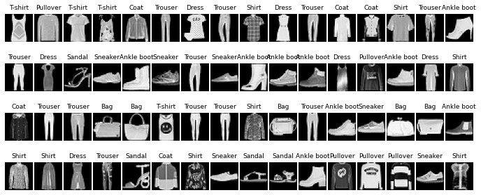
# Visualize an image of a batch
batch_x = b_x.squeeze().numpy()
batch_y = b_y.numpy()
label = train_data.classes
label[0] = 'T-shirt'
plt.figure(figsize = (12, 5))
for i in np.arange(len(batch_y)):
plt.subplot(4, 16, i + 1)
plt.imshow(batch_x[i, :, :], cmap = plt.cm.gray)
plt.title(label[batch_y[i]], size = 9)
plt.axis('off')
plt.subplots_adjust(wspace = 0.05)
# Processing Test Sets
test_data = FashionMNIST(
root = './data/FashionMNIST',
train = False, # Do not use training datasets
download = False
)
# Add a channel dimension to the data and normalize the range of values
test_data_x = test_data.data.type(torch.FloatTensor) / 255.0
test_data_x = torch.unsqueeze(test_data_x, dim = 1)
test_data_y = test_data.targets # Test Set Label
print(test_data_x.shape)
print(test_data_y.shape)
938
torch.Size([10000, 1, 28, 28])
torch.Size([10000])
# Define hollow network objects
myconvdilanet = MyConvDilaNet()
from torchsummary import summary
summary(myconvdilanet, input_size=(1, 28, 28))
----------------------------------------------------------------
        Layer (type)               Output Shape         Param #
================================================================
            Conv2d-1           [-1, 16, 26, 26]             160
              ReLU-2           [-1, 16, 26, 26]               0
         AvgPool2d-3           [-1, 16, 13, 13]               0
            Conv2d-4             [-1, 32, 9, 9]           4,640
              ReLU-5             [-1, 32, 9, 9]               0
         AvgPool2d-6             [-1, 32, 4, 4]               0
            Linear-7                  [-1, 256]         131,328
              ReLU-8                  [-1, 256]               0
            Linear-9                  [-1, 128]          32,896
             ReLU-10                  [-1, 128]               0
           Linear-11                   [-1, 10]           1,290
================================================================
Total params: 170,314
Trainable params: 170,314
Non-trainable params: 0
----------------------------------------------------------------
Input size (MB): 0.00
Forward/backward pass size (MB): 0.24
Params size (MB): 0.65
Estimated Total Size (MB): 0.89
----------------------------------------------------------------
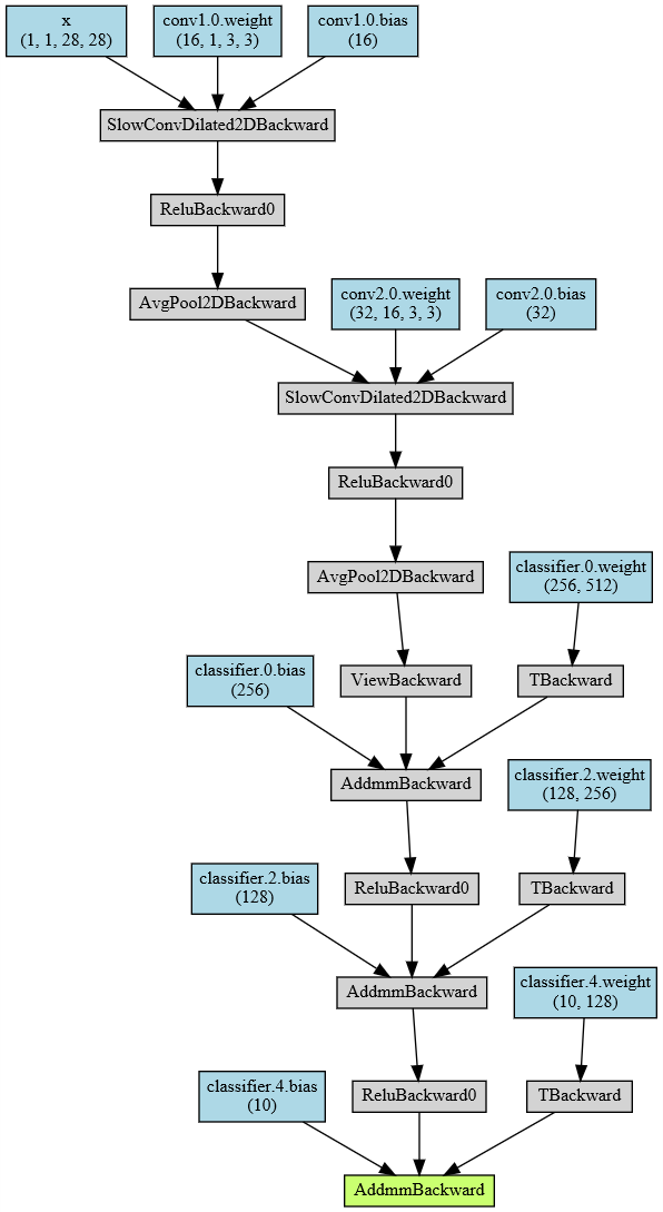
# Output Network Structure
from torchviz import make_dot

x = torch.randn(1, 1, 28, 28).requires_grad_(True)
y = myconvdilanet(x)
myDilaCNN_vis = make_dot(y, params=dict(list(myconvdilanet.named_parameters()) + [('x', x)]))
myDilaCNN_vis
Training and Prediction of Hole Convolution Neural Network
The network training and testing section is the same as above.
# Define network training process functions
def train_model(model, traindataloader, train_rate, criterion, optimizer, num_epochs = 25):
    '''
    Model, training dataset(To be sliced),Percentage of training set, loss function, optimizer, number of training rounds
    '''
    # Calculate the number of batch es used for training
    batch_num = len(traindataloader)
    train_batch_num = round(batch_num * train_rate)
    # Copy model parameters
    best_model_wts = copy.deepcopy(model.state_dict())
    best_acc = 0.0
    train_loss_all = []
    val_loss_all =[]
    train_acc_all = []
    val_acc_all = []
    since = time.time()
    # Training Framework
    for epoch in range(num_epochs):
        print('Epoch {}/{}'.format(epoch, num_epochs - 1))
        print('-' * 10)
        train_loss = 0.0
        train_corrects = 0
        train_num = 0
        val_loss = 0.0
        val_corrects = 0
        val_num = 0
        for step, (b_x, b_y) in enumerate(traindataloader):
            if step < train_batch_num:
                model.train()   # Set as training mode
                output = model(b_x)
                pre_lab = torch.argmax(output, 1)
                loss = criterion(output, b_y)   # Calculating Error Loss
                optimizer.zero_grad()   # Empty Past Gradient
                loss.backward() # Error Back Propagation
                optimizer.step()    # Update parameters based on errors
                train_loss += loss.item() * b_x.size(0)
                train_corrects += torch.sum(pre_lab == b_y.data)
                train_num += b_x.size(0)
            else:
                model.eval()    # Set to Verification Mode
                output = model(b_x)
                pre_lab = torch.argmax(output, 1)
                loss = criterion(output, b_y)
                val_loss += loss.item() * b_x.size(0)
                val_corrects += torch.sum(pre_lab == b_y.data)
                val_num += b_x.size(0)
        # ==========================End of small loop=======================End of small loop==========

        # Calculate loss and accuracy of an epoch on training and validation sets
        train_loss_all.append(train_loss / train_num)
        train_acc_all.append(train_corrects.double().item() / train_num)
        val_loss_all.append(val_loss / val_num)
        val_acc_all.append(val_corrects.double().item() / val_num)
        print('{} Train Loss: {:.4f} Train Acc: {:.4f}'.format(epoch, train_loss_all[-1], train_acc_all[-1]))
        print('{} Val Loss: {:.4f} Val Acc: {:.4f}'.format(epoch, val_loss_all[-1], val_acc_all[-1]))

        # Parameters with the highest precision of the copy model
        if val_acc_all[-1] > best_acc:
            best_acc = val_acc_all[-1]
            best_model_wts = copy.deepcopy(model.state_dict())
        time_use = time.time() - since
        print('Train and Val complete in {:.0f}m {:.0f}s'.format(time_use // 60, time_use % 60))
    # ===============================End of Big Loop==========================


    # Parameters using the best model
    model.load_state_dict(best_model_wts)
    train_process = pd.DataFrame(
        data = {'epoch': range(num_epochs),
                'train_loss_all': train_loss_all,
                'val_loss_all': val_loss_all,
                'train_acc_all': train_acc_all,
                'val_acc_all': val_acc_all})
    return model, train_process
# Training the model
optimizer = Adam(myconvdilanet.parameters(), lr = 0.0003)
criterion = nn.CrossEntropyLoss()
myconvdilanet, train_process = train_model(myconvdilanet, train_loader, 0.8, criterion, optimizer, num_epochs = 25)
Epoch 0/24
----------
0 Train Loss: 0.8922 Train Acc: 0.6718
0 Val Loss: 0.6322 Val Acc: 0.7498
Train and Val complete in 1m 2s
Epoch 1/24
----------
1 Train Loss: 0.6028 Train Acc: 0.7656
1 Val Loss: 0.5610 Val Acc: 0.7837
Train and Val complete in 2m 3s
Epoch 2/24
----------
2 Train Loss: 0.5331 Train Acc: 0.7948
2 Val Loss: 0.5047 Val Acc: 0.8107
Train and Val complete in 3m 3s
Epoch 3/24
----------
3 Train Loss: 0.4868 Train Acc: 0.8159
3 Val Loss: 0.4738 Val Acc: 0.8266
Train and Val complete in 3m 60s
Epoch 4/24
----------
4 Train Loss: 0.4540 Train Acc: 0.8320
4 Val Loss: 0.4491 Val Acc: 0.8369
Train and Val complete in 4m 54s
Epoch 5/24
----------
5 Train Loss: 0.4275 Train Acc: 0.8433
5 Val Loss: 0.4279 Val Acc: 0.8455
Train and Val complete in 5m 50s
Epoch 6/24
----------
6 Train Loss: 0.4047 Train Acc: 0.8512
6 Val Loss: 0.4075 Val Acc: 0.8531
Train and Val complete in 6m 45s
Epoch 7/24
----------
7 Train Loss: 0.3851 Train Acc: 0.8591
7 Val Loss: 0.3897 Val Acc: 0.8608
Train and Val complete in 7m 41s
Epoch 8/24
----------
8 Train Loss: 0.3690 Train Acc: 0.8655
8 Val Loss: 0.3762 Val Acc: 0.8653
Train and Val complete in 8m 36s
Epoch 9/24
----------
9 Train Loss: 0.3557 Train Acc: 0.8708
9 Val Loss: 0.3652 Val Acc: 0.8672
Train and Val complete in 9m 31s
Epoch 10/24
----------
10 Train Loss: 0.3440 Train Acc: 0.8751
10 Val Loss: 0.3552 Val Acc: 0.8710
Train and Val complete in 10m 26s
Epoch 11/24
----------
11 Train Loss: 0.3341 Train Acc: 0.8776
11 Val Loss: 0.3473 Val Acc: 0.8735
Train and Val complete in 11m 22s
Epoch 12/24
----------
12 Train Loss: 0.3250 Train Acc: 0.8812
12 Val Loss: 0.3412 Val Acc: 0.8762
Train and Val complete in 12m 21s
Epoch 13/24
----------
13 Train Loss: 0.3166 Train Acc: 0.8840
13 Val Loss: 0.3355 Val Acc: 0.8791
Train and Val complete in 13m 25s
Epoch 14/24
----------
14 Train Loss: 0.3092 Train Acc: 0.8870
14 Val Loss: 0.3299 Val Acc: 0.8810
Train and Val complete in 14m 26s
Epoch 15/24
----------
15 Train Loss: 0.3023 Train Acc: 0.8889
15 Val Loss: 0.3250 Val Acc: 0.8816
Train and Val complete in 15m 28s
Epoch 16/24
----------
16 Train Loss: 0.2956 Train Acc: 0.8921
16 Val Loss: 0.3182 Val Acc: 0.8838
Train and Val complete in 16m 30s
Epoch 17/24
----------
17 Train Loss: 0.2896 Train Acc: 0.8939
17 Val Loss: 0.3138 Val Acc: 0.8862
Train and Val complete in 17m 32s
Epoch 18/24
----------
18 Train Loss: 0.2836 Train Acc: 0.8961
18 Val Loss: 0.3093 Val Acc: 0.8872
Train and Val complete in 18m 33s
Epoch 19/24
----------
19 Train Loss: 0.2783 Train Acc: 0.8984
19 Val Loss: 0.3054 Val Acc: 0.8894
Train and Val complete in 19m 34s
Epoch 20/24
----------
20 Train Loss: 0.2728 Train Acc: 0.9004
20 Val Loss: 0.3020 Val Acc: 0.8911
Train and Val complete in 20m 52s
Epoch 21/24
----------
21 Train Loss: 0.2676 Train Acc: 0.9021
21 Val Loss: 0.2989 Val Acc: 0.8922
Train and Val complete in 21m 54s
Epoch 22/24
----------
22 Train Loss: 0.2625 Train Acc: 0.9038
22 Val Loss: 0.2960 Val Acc: 0.8942
Train and Val complete in 22m 55s
Epoch 23/24
----------
23 Train Loss: 0.2578 Train Acc: 0.9049
23 Val Loss: 0.2932 Val Acc: 0.8942
Train and Val complete in 23m 56s
Epoch 24/24
----------
24 Train Loss: 0.2531 Train Acc: 0.9062
24 Val Loss: 0.2907 Val Acc: 0.8942
Train and Val complete in 24m 58s
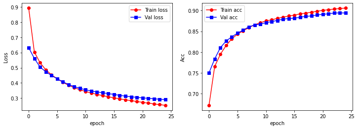
Visualize the training process using line charts:
# Visual training process
plt.figure(figsize = (12, 4))
plt.subplot(1, 2, 1)
plt.plot(train_process.epoch, train_process.train_loss_all, 'ro-', label = 'Train loss')
plt.plot(train_process.epoch, train_process.val_loss_all, 'bs-', label = 'Val loss')
plt.legend()
plt.xlabel('epoch')
plt.ylabel('Loss')

plt.subplot(1, 2, 2)
plt.plot(train_process.epoch, train_process.train_acc_all, 'ro-', label = 'Train acc')
plt.plot(train_process.epoch, train_process.val_acc_all, 'bs-', label = 'Val acc')
plt.legend()
plt.xlabel('epoch')
plt.ylabel('Acc')

plt.show()
Compute the generalization ability of the void convolution model:
# Test Set Prediction and Visualize Prediction Effect
myconvdilanet.eval()
output = myconvdilanet(test_data_x)
pre_lab = torch.argmax(output, 1)
acc = accuracy_score(test_data_y, pre_lab)
print(test_data_y)
print(pre_lab)
print('The prediction accuracy on the test set is', acc)
tensor([9, 2, 1,  ..., 8, 1, 5])
tensor([9, 2, 1,  ..., 8, 1, 5])
Prediction accuracy on test set is 0.8841
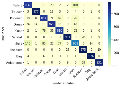
Using thermograms, observe the predictions on each type of data:
# Compute and visualize confusion matrices on test sets
conf_mat = confusion_matrix(test_data_y, pre_lab)
df_cm = pd.DataFrame(conf_mat, index = label, columns = label)
heatmap = sns.heatmap(df_cm, annot = True, fmt = 'd', cmap = 'YlGnBu')
heatmap.yaxis.set_ticklabels(heatmap.yaxis.get_ticklabels(), rotation = 0, ha = 'right')
heatmap.xaxis.set_ticklabels(heatmap.xaxis.get_ticklabels(), rotation = 45, ha = 'right')
plt.ylabel('True label')
plt.xlabel('Predicted label')
plt.show()